Linear and nonlinear receptivity mechanisms in boundary layers subject to free-stream turbulence

Abstract

Large-eddy simulations of a flat-plate boundary layer, without a leading edge, subject to multiple levels of incoming free-stream turbulence are considered in the present work. Within an input–output model, where nonlinear terms of the incompressible Navier–Stokes equations are treated as an external forcing, we manage to separate inputs related to perturbations coming through the intake of the numerical domain, whose evolution represents a linear mechanism, and the volumetric nonlinear forcing due to triadic interactions. With these, we perform the full reconstruction of the statistics of the flow, as measured in the simulations, to quantify pairs of wavenumbers and frequencies more affected by either linear or nonlinear receptivity mechanisms. Inside the boundary layer, different wavenumbers at near-zero frequency reveal streaky structures. Those that are amplified predominantly via linear interactions with the incoming vorticity occur upstream and display transient growth, while those generated by the nonlinear forcing are the most energetic and appear in more downstream positions. The latter feature vortices growing proportionally to the laminar boundary layer thickness, along with a velocity profile that agrees with the optimal amplification obtained by linear transient growth theory. The numerical approach presented is general and could potentially be extended to any simulation for which receptivity to incoming perturbations needs to be assessed.

1. Introduction

Boundary-layer flows are among the most studied problems in fluid dynamics due to their practical importance in the determination of the skin-friction drag of objects, heat transfer and stall characteristics in airplane wings and turbine blades.

Nevertheless, to this day, there is no general mathematical model capable of predicting the transition from laminar to turbulent flow under all conditions, even for the simplest case of a boundary layer over a flat plate without pressure gradient (Saric, Reed & Kerschen 2002; Fransson & Shahinfar 2020). This unpredictability is mainly due to the multiple parameters that are known to affect transition, such as free-stream turbulence intensity, sound, surface roughness, leading-edge shape and the still incomplete knowledge of how these parameters interact.

Concerning environmental effects, a simplified roadmap to turbulence is described by Morkovin, Reshotko & Herbert (1994) as a function of disturbance amplitudes, with transition beginning with the process denoted receptivity (Morkovin 1969), in which wave-like disturbances originating in the free flow enter the boundary layer.

If the magnitude of environmental disturbances is weak, the initial growth of the boundary-layer instabilities can be described by modal stability theory, which predicts the exponential evolution of the primary unstable modes (eigenfunctions) of the Orr–Sommerfeld–Squire (OSS) equations over relatively long lengths (Reed, Saric & Arnal 1996). In the boundary layer over flat plates, subject to no pressure gradient, these primary instabilities are two-dimensional oscillatory modes called Tollmien–Schlichting (TS) waves (Schubauer & Skramstad 1947). Then, at large enough perturbation amplitudes, nonlinear effects take place and the unstable linear modes lose symmetry, degenerating into secondary instabilities before breaking into turbulent spots due to nonlinear mechanisms.

On the other hand, in the presence of stronger environmental forcing, turbulent spots inside the boundary layer appear much sooner than predicted by modal stability, completely bypassing primary mode growth. This phenomenon, therefore called bypass transition (Morkovin 1969, 1985), has since been associated with cases such as rough surfaces (Reshotko 1984; Morkovin 1990; Denissen & White 2008; von Deyn et al. 2020) and high free-stream turbulence levels, above around 1 % (Morkovin 1985; Suder, Obrien & Reshotko 1988; Matsubara & Alfredsson 2001), where linear theory predictions fail and receptivity mechanisms are still not well understood.

Initially, bypass transition was thought to be mainly a result of nonlinear phenomena, a notion that was later challenged by the concept of transient growth (Reshotko 2001), developed in the early 1990s and formalised in Schmid et al. (1993). Due to the non-orthogonality of the OSS operator, the superposition of eigenfunctions can lead to a transient algebraic growth, even in cases where the boundary layer is linearly stable, i.e. below the critical Reynolds number for the occurrence of TS waves.

Transient growth theory, often referred to as non-modal stability theory, is based on the lift-up effect first demonstrated by Ellingsen & Palm (1975) and later developed by Landahl (1980), where three-dimensional infinitesimal disturbances can grow algebraically in parallel inviscid shear flows, regardless of the modal stability conditions. Moreover, Landahl (1980) formally connected this behaviour with the low frequency longitudinal streaky structures first identified in transitional and turbulent boundary layers by Klebanoff (1971), later found to be important in all transitional and turbulent shear flows (Brandt 2014). The magnitude of the transient growth is an important parameter that defines the path to turbulence. Weaker streaks may simply decay, giving space to primary mode growth, or lead to secondary instabilities. Stronger streaks, however, might degenerate directly into turbulent spots.

In the specific case of bypass transition in boundary layers due to free-stream turbulence (FST), two distinct receptivity mechanisms have been proposed (Brandt, Schlatter & Henningson 2004): a linear mechanism caused by perturbations at the leading edge and a nonlinear one, caused by interactions between oblique waves above the boundary layer.

When vortical disturbances are present at the leading edge, low-frequency perturbations induce streamwise vortices of alternating direction that, in turn, cause the linear transient growth of streaky structures inside the laminar boundary layer (Butler & Farrell 1992; Andersson, Berggren & Henningson 1999; Luchini 2000). These streaks are characterised by alternating regions of fast and slow longitudinal flow. In locations where the streamwise vortices carry matter downwards to the wall, a fast (positive) streak is generated, while the outflow from the wall generates slow (negative) streaks. The profiles for the optimal response of streaks induced by this mechanism consistently match experiments (Kendall 1998; Matsubara & Alfredsson 2001), as discussed by Luchini (2000).

On the other hand, when disturbances are found above the boundary layer, the transition can be triggered by pairs of oblique waves propagating at the same frequency, $\omega$, and opposite spanwise wavenumbers, $\pm \beta$, generating structures in the boundary layer, through quadratic nonlinear interactions, which are associated with double the initial wavenumber, i.e. $(\pm \beta,\omega ) \rightarrow (2\beta,0)$. This mechanism is also known to generate streamwise vortices and streaks (Schmid, Reddy & Henningson 1996), a process verified both numerically and experimentally (Berlin, Wiegel & Henningson 1999) and modelled via weakly nonlinear analysis (Brandt, Henningson & Ponziani 2002).

In this work, a set of numerical simulations of a boundary layer subject to different levels of FST is considered, to study in detail the process of receptivity to external vorticity. Modal analysis, namely spectral proper orthogonal decomposition (POD) (Towne, Schmidt & Colonius 2018), and resolvent analysis (Jovanović & Bamieh 2005; McKeon & Sharma 2010) are employed, in combination with the ideas developed in Morra et al. (2021) and Nogueira et al. (2021) which, in turn, arise from the realisation that accurate predictions from linear models require accurate knowledge of the nonlinear forcing statistics (Chevalier et al. 2006), which would otherwise be modelled as incoherent (white) noise (Hæpffner et al. 2005). The coloured statistics of the nonlinear forcing term are computed directly from the simulated data and, instead of computing spectral POD modes of the forcing, we obtain, via the resolvent-based extended spectral POD method (Karban et al. 2022), response and forcing modes which are related by the resolvent operator. This set-up allows for the identification of coherent structures that are more affected by either linear or nonlinear interactions with vortical free-stream disturbances of a complex nature. In the latter case, the nonlinear forcing capable of generating said coherent structures is characterised.

The separated consideration of linear and nonlinear mechanisms in the resolvent framework allows us to explore how streaks present in the data can be connected to upstream disturbances through a linear receptivity, or to triadic interactions in a nonlinear receptivity. The dominance of each mechanism in different regions of the boundary layer may thus be quantified using simulation data.

This manuscript is divided in the following manner: § 2 describes in detail the numerical set-up employed in the study; § 3 exposes the mathematical formulation capable of separating linear and nonlinear receptivity mechanisms and the spectral analysis procedures; §§ 4–8.3 present and discuss the results, discussing the differences found between linearly and nonlinearly induced structures inside and outside the boundary layer. The manuscript is completed with conclusions in § 9.

2. Boundary-layer simulations

We performed multiple simulations of boundary-layer flows subject to different levels of FST $Tu$, varying from $Tu=0.5\,\%$ to $3.5\,\%$, in steps of $0.5\,\%$, for a total of seven different cases. The databases were obtained using the SIMSON pseudo-spectral solver (Chevalier, Lundbladh & Henningson 2007). These are large-eddy simulations (LES) of transitional regimes in a Blasius-type boundary layer over a flat plate without a leading edge and zero pressure gradient, performed using an approximate deconvolution model with relaxation terms (Stolz, Adams & Kleiser 2001; Schlatter, Stolz & Kleiser 2006).

2.1. Numerical set-up

Each simulation was set according to Sasaki et al. (2020), based on the work of Brandt et al. (2004), and consists of a $231 \times 121 \times 108 (x \times y \times z)$ Cartesian grid constructed with Chebyshev nodes in the $y$ direction, perpendicular to the wall, and homogeneously spaced nodes in the streamwise and spanwise directions, $x$ and $z$. The boundary layer is started with a finite thickness. All variables are non-dimensionalised by the reference length $\delta ^*_0$, the boundary-layer displacement thickness at the intake, and a time scale $t = \delta ^*_0/U_\infty$, where $U_\infty$ is the free-stream velocity. The numerical domain is a box of size $x \in [0,1000]$, $y \in [0,60]$ and $z \in [-25,25]$. Both the $x$ and $z$ directions are periodic and decomposed in Fourier modes, while the $y$ direction uses a Chebyshev polynomial basis. Periodicity in the streamwise direction is achieved by the introduction of a fringe region contained in the range $x \in [910,1000]$.

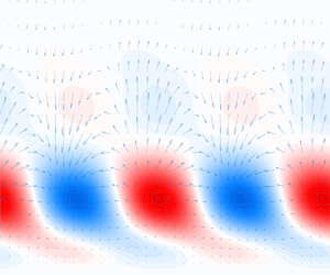
At the intake, $Re_{\delta _0^*}= U_\infty \delta ^*_0/\nu = 300$, with $\nu$ being the kinematic viscosity of the fluid. At this Reynolds number, the boundary layer is linearly stable and, thus, TS waves are not expected to be significant over the relatively short extent of the domain. Instead, streamwise elongated (streaky) structures are observed in the simulations at the highest FST levels investigated, as shown in figure 1.

Figure 1. Snapshot of a simulation with $Tu=3.5\,\%$ incoming FST level, where streaky structures can be identified. Slice at $y = 0.8$, inside the boundary layer.

The no-slip condition

(2.1)\begin{equation} \boldsymbol{u^\prime}(x,0,z,t) = 0, \end{equation}

is imposed on the wall and the Neumann condition

(2.2)\begin{equation} \frac{\partial}{\partial y} \boldsymbol{u^\prime}(x,60,z,t) = 0, \end{equation}

is applied on the upper boundary, with $\boldsymbol {u^\prime }(x,y,z,t)$ representing velocity fluctuations with respect to the two-dimensional Blasius base flow, $\boldsymbol {U}_{BL}(x,y)$ (figure 2). For all performed simulations, the physical domain ends before the development of turbulent spots in the boundary layer, i.e. before the transition to the turbulent regime. The use of a short spatial domain reduces the computational cost of the present study, which involves detailed post-processing of several numerical simulations. Moreover, by restricting the domain to the initial development of streaks we can focus on the receptivity stage, before the actual transition to turbulence that would occur at larger values of $x$.

Figure 2. Diagram of the boundary-layer set-up, showing boundary conditions. The $x$ and $z$ directions are periodic and $\delta _0$ is the initial boundary-layer thickness. Here, $\boldsymbol {U_{BL}}(x,y)$ is the Blasius base flow and $\boldsymbol {u^\prime }(x,y,z)$ are velocity fluctuations. Legend: (dotted line) forcing modes from the continuous branch of the OSS operator.

Concerning the time evolution, linear terms of the Navier–Stokes (NS) equations are implicitly marched with a second-order Crank–Nicolson scheme, while an explicit third-order, four-stage, Runge–Kutta scheme is applied over nonlinear terms. For each simulation, we compute a total of 2000 snapshots, taken in time steps of $\Delta t=10$, of fully developed, statistically stationary, flow.

2.2. Fringe region forcing

Some assumptions are made to synthesise valid inflow conditions at $x=0$ and circumvent the need to compute a turbulent field upstream of the flat plate or the flow around a leading edge. Isotropic and homogeneous FST is introduced in the simulations by forcing several modes in the continuous branch of the linearised OSS operator within the fringe region, as illustrated in figure 2.

The FST generation procedure is referred to in Schlatter (2001) and Brandt et al. (2004), based on the methods presented in Grosch & Salwen (1978) and Jacobs & Durbin (2001). Considering the linearised NS (LNS) momentum equations in perturbation form around a base flow and nonlinear fluctuation terms gathered into the function $f(\boldsymbol {u^\prime })$, we force a desired velocity vector $\boldsymbol {\zeta }(x,y,z,t)$ inside the fringe following the formulation

(2.3)\begin{equation} \left. \begin{array}{c@{}} \dfrac{\partial \boldsymbol{u^\prime}}{\partial t} = LNS (\boldsymbol{u^\prime},\boldsymbol{U_{BL}}) + {f(\boldsymbol{u^\prime})} + \sigma(x)(\boldsymbol{\zeta}-\boldsymbol{u^\prime}),\\ \boldsymbol{\nabla} \boldsymbol{\cdot} \boldsymbol{u^\prime} = 0, \end{array}\right\} \end{equation}

where $\sigma (x)$ is a gain function, which is positive inside the fringe region and null everywhere else (figure 3). The term $\sigma (x)(\boldsymbol {\zeta }-\boldsymbol {u^\prime })$ is thus responsible for smoothly changing the fluctuation field entering the left side of the fringe region towards the desired reference forcing vector $\boldsymbol {\zeta }$ introduced in the fringe.

Figure 3. Fringe gain function, the same as that described in Chevalier et al. (2007). The maximum gain inside the fringe is set to 0.8.

Isotropic homogeneous turbulence can be represented as a sum of Fourier modes with random amplitude (Rogallo 1981). In the boundary-layer case, however, this approach is not capable of modelling the presence of the wall, as the $y$ direction is non-homogeneous. For this application, a basis composed of modes in the continuous spectrum of the OSS operator is assumed to be a reasonable choice to satisfy all the necessary boundary conditions. These modes tend to Fourier modes far from the wall and decay to zero near it, generating a perturbation field mainly localised outside the boundary layer, as shown in Appendix A. On the other hand, modes of the discrete spectrum are only significant inside the boundary layer and decay exponentially farther from the wall, not being suitable in this application (Grosch & Salwen 1978).

By computing eigenfunctions in the continuous branch of the OSS spectrum, $\boldsymbol {u^\prime _{OSS}}$, normalised to unit energy, we can write the expansion for an arbitrary perturbation vector

(2.4)\begin{equation} \boldsymbol{\zeta}(x,y,z,t) = {\rm Re}\left\{\sum_{\omega} \sum_{\gamma} \sum_{\beta} \varPhi(\omega,\gamma,\beta) \boldsymbol{u^\prime_{OSS}}(\omega,y,\beta) \, {\rm e}^{{\rm i}({\rm Re}\{\alpha(\omega,\gamma,\beta)\} x + \beta z - \omega t )}\right\}, \end{equation}

where $\omega$, $\gamma$ and $\beta$ are real parameters and $\alpha (\omega,\gamma,\beta )$ is the complex eigenvalue of $\boldsymbol {u^\prime _{OSS}}$ computed via spatial stability (Jacobs & Durbin 2001). Here, $\alpha,\gamma,\beta$ are respectively the wavenumbers in the $x,y,z$ directions and $\omega$ the frequency. The factor $\varPhi$ is the energy scaling applied to match the von Kármán spectrum, discussed in the following paragraphs. Only the real part of $\alpha$ is taken inside the exponent to maintain the forcing fluctuation at a fixed magnitude throughout the fringe zone's streamwise extension, ignoring in practice the effects of viscous attenuation (Brandt et al. 2004).

We consider wavenumbers $\kappa = \sqrt {\textrm {Re}\{\alpha \}^2+\gamma ^2+\beta ^2}$ equally spaced within the range limited by the numerical resolution of the simulations, $\kappa \in [\kappa _l,\kappa _u]$. In general, $\kappa _l$ is a function of the domain size, while $\kappa _u$ is bounded by the resolution of the grid. For simplification, we replace $\omega = \alpha U_\infty$, considering that modes of the continuous spectrum have phase speed equal to $U_\infty$, to define a tridimensional space of parameters $(\omega,\gamma,\beta )$ for which a given value $\kappa$ is represented by a spherical shell (Brandt et al. 2004). We select $N_s$ shells, within which we include $N_\kappa$ combinations of the $(\omega,\gamma,\beta )$ parameters of constant $\kappa$, filling the surface with equally spaced points (Schlatter 2001). The value $\gamma =0$ is avoided. A random rotation is applied to each shell at every time step to further improve isotropy. In this work, we adopt the values $\kappa _l=0.23$, $\kappa _u=3.0$, $N_s = 20$ and $N_\kappa = 10$, in a total of $N_s N_\kappa = 200$ eigenfunctions, the same as in Sasaki et al. (2020).

Once the suitable modes are chosen, the energy scale needs to be applied. Considering the von Kármán spectrum for isotropic homogeneous turbulence and following the three-dimensional spectrum construction in Tennekes & Lumley (1972), we have the formula for turbulent energy as a function of wavenumber

(2.5)\begin{equation} E(\kappa) = \frac{2}{3} \frac{a (\kappa L)^4}{(b + (\kappa L)^2 )^{{17}/{6}}} L \cdot Tu^2, \quad L = \frac{1.8}{\kappa_{max}}, \end{equation}

where $a = 1.606$, $b = 1.35$ and $Tu$ is the turbulence intensity level defined as

(2.6)\begin{equation} Tu = \sqrt{\frac{(u'^2_{rms}+v'^2_{rms}+w'^2_{rms})}{3}}. \end{equation}

In this equation, the integral length scale $L=7.5 \delta _0^*$ is set to the same value considered in Sasaki et al. (2020), yielding a wavenumber of maximum energy, $\kappa _{max}$, near the minimum allowed value of $\kappa _l$. According to the results shown in Brandt et al. (2004), the increase of the turbulence integral length reduces the turbulence intensity decay at the free stream and promotes transition in positions further upstream. Therefore, this choice of integral length scale consists of a worst case scenario, which allows a shorter domain size in the streamwise direction.

Concerning the energy scaling, it is demonstrated in Schlatter (2001) that the factor $\varPhi$ in (2.4) can be then expressed as

(2.7)\begin{equation} \varPhi(\kappa) = \sqrt{\frac{E(\kappa) \Delta \kappa}{N_s}}, \end{equation}

where $\Delta \kappa$ is the difference between consecutive values of $\kappa$.

Finally, the amplitudes of OSS modes in the continuous branch of the spectrum must be addressed at the top boundary of the domain. To prevent numerical instabilities, we multiply the eigenfunctions by a smooth step function $S(\kern0.7pt y)$ (Brandt et al. 2004) to dampen forcing perturbations above the position $y_d = 0.8 y_{max}$.

A more detailed discussion concerning the properties of the inflow perturbations generated using OSS modes in the continuous branch is presented in Appendix A.

3. Analysis techniques

3.1. Input–output formulation

To apply the resolvent analysis framework over NS equations, we separate the velocity field into a two-dimensional, time-invariant, laminar solution (Jovanović & Bamieh 2005) or ensemble average flow (McKeon & Sharma 2010)

(3.1)\begin{equation} \boldsymbol{U} = [U(x,y),V(x,y),0]^T, \end{equation}

and fluctuations

(3.2)\begin{equation} \boldsymbol{u^\prime} = [u^\prime(x,y,z,t),v^\prime(x,y,z,t),w^\prime(x,y,z,t)]^T, \end{equation}

in order to write the linearised equations around $\boldsymbol {U}$, as described in (2.3). Using tensor formulation, the system can be written as

(3.3)\begin{equation} \left. \begin{array}{c@{}} \displaystyle \dfrac{\partial u^\prime_i}{\partial t} + U_j \dfrac{\partial u^\prime_i}{\partial x_j} + u^\prime_j \dfrac{\partial U_i}{\partial x_j} ={-} \dfrac{\partial p^\prime}{\partial x_i} + \dfrac{1}{Re} \dfrac{\partial^2 u^\prime_i}{\partial x_j \partial x_j} + f_i + \sigma(\zeta_i - u^\prime_i), \\ \displaystyle \dfrac{\partial u^\prime_j}{\partial x_j} = 0, \end{array}\right\} \end{equation}

with nonlinear terms grouped in $f_i = - u^\prime _j ({\partial u^\prime _i}/{\partial x_j})$, considered in the resolvent framework as a forcing that drives the linear dynamics. The term $\zeta _i$ is the forcing vector defined in (2.3), which guarantees that inlet conditions in the model statistically match those observed in the boundary-layer simulations. The function $\sigma (x)$ is the same as presented in figure 3.

Next, we apply the normal mode ansatz $\boldsymbol {u^\prime } = \hat {\boldsymbol {u}}(x,y) \, \textrm {e}^{\textrm {i} (\beta z - \omega t)}$ over the velocity, pressure and forcing fields to expand (3.3) as

(3.4) \begin{align} \left. \begin{array}{c@{}} \displaystyle -{\rm i} \omega \hat{u} + U \dfrac{\partial \hat{u}}{\partial x} + V \dfrac{\partial \hat{u}}{\partial y} + \hat{u} \dfrac{\partial U}{\partial x} + \hat{v} \dfrac{\partial U}{\partial y} + \dfrac{\partial \hat{p}}{\partial x} - \dfrac{1}{Re}\left(\dfrac{\partial^2}{\partial x^2} -\beta^2 + \dfrac{\partial^2}{\partial y^2} \right) \hat{u} = \hat{f}_x + \sigma (\hat{\zeta}_x-\hat{u}), \\ \displaystyle -{\rm i} \omega \hat{v} + U \dfrac{\partial \hat{v}}{\partial x} + V \dfrac{\partial \hat{v}}{\partial y} + \hat{u} \dfrac{\partial V}{\partial x} + \hat{v} \dfrac{\partial V}{\partial y} + \dfrac{\partial \hat{p}}{\partial y} - \dfrac{1}{Re}\left(\dfrac{\partial^2}{\partial x^2} -\beta^2 + \dfrac{\partial^2}{\partial y^2} \right) \hat{v} = \hat{f}_y + \sigma (\hat{\zeta}_y-\hat{v}), \\ \displaystyle -{\rm i} \omega \hat{w} + U \dfrac{\partial \hat{w}}{\partial x} + V \dfrac{\partial \hat{w}}{\partial y} + {\rm i} \beta \hat{p} + \dfrac{1}{Re} \left(\dfrac{\partial^2}{\partial x^2} -\beta^2 + \dfrac{\partial^2}{\partial y^2} \right) \hat{w} = \hat{f}_z + \sigma (\hat{\zeta}_z-\hat{w}), \\ \displaystyle \dfrac{\partial \hat{u}}{\partial x} + \dfrac{\partial \hat{v}}{\partial y} + {\rm i} \beta \hat{w} = 0, \end{array} \right\} \end{align}

where the nonlinear term $\widehat {f_i}$ can be written as a convolution of the Fourier transform of velocity components

(3.5)\begin{equation} \widehat{f_i}(\beta,\omega) ={-} \hat{u}_j \ast \frac{\partial \hat{u}_i}{\partial x_j} ={-} \int_{-\infty}^{\infty} \int_{-\infty}^{\infty} \hat{u}_j(\beta_0,\omega_0) \frac{\partial }{\partial x_j} \hat{u}_i(\beta-\beta_0,\omega-\omega_0) \, {\rm d} \beta_0 \, {\rm d} \omega_0. \end{equation}

This implies that $\widehat {f_i}$ are the only terms responsible for energy transfers between different wavenumbers ($\beta,\beta _0,\beta -\beta _0$) and frequencies ($\omega,\omega _0,\omega -\omega _0$), in triads related to the turbulent energy cascade (Cheung & Zaki 2014; Moffatt 2014).

In practice, the fringe perturbation vector in Fourier space, $\hat {\boldsymbol {\zeta }}$, is approximated by the velocity fluctuation field computed from the simulations, denoted as $\hat {\boldsymbol {u}}_{\boldsymbol r}$, which is substituted in (3.4) for all three spatial components. Next, this equation is discretised reproducing the same grid of the LES and equivalent boundary conditions to write the system in state-space form

(3.6)\begin{equation} \left. \begin{array}{c@{}} (\boldsymbol{\varOmega}+{\boldsymbol{\mathsf{L}}}) \hat{\boldsymbol{q}} = {\boldsymbol{\mathsf{B}}}_{{\boldsymbol{\mathsf{u}}}} \hat{\boldsymbol{u}}_{\boldsymbol r} + {\boldsymbol{\mathsf{B}}}_{\boldsymbol{\mathsf{f}}} \hat{\boldsymbol{f}}, \\ \hat{\boldsymbol{y}} = {\boldsymbol{\mathsf{H}}} \hat{\boldsymbol{q}}, \end{array} \right\}, \end{equation}

and obtain

(3.7)\begin{equation} {\boldsymbol{\mathsf{R}}} = {\boldsymbol{\mathsf{H}}}(\boldsymbol{\varOmega}+{\boldsymbol{\mathsf{L}}})^{{-}1} \implies \hat{\boldsymbol{y}} = {\boldsymbol{\mathsf{R}}} ({\boldsymbol{\mathsf{B}}}_{{\boldsymbol{\mathsf{u}}}} \hat{\boldsymbol{u}}_{\boldsymbol r} + {\boldsymbol{\mathsf{B}}}_{\boldsymbol{\mathsf{f}}} \hat{\boldsymbol{f}}), \end{equation}

where ${\boldsymbol{\mathsf{R}}}$ is the resolvent operator and $\hat {\boldsymbol {q}} = [\hat {u},\hat {v},\hat {w},\hat {p}]^T$, $\hat {\boldsymbol {y}} = [\hat {u},\hat {v},\hat {w}]^T$, $\hat {\boldsymbol {u}}_{\boldsymbol r} = [\hat {u}_r,\hat {v}_r,\hat {w}_r]^T$, $\hat{\boldsymbol{f}} = [\,\hat{f}_x,\hat{f}_y,\hat{f}_z]^T$ are vectors composed of row-wise stacked components. Operators $\boldsymbol {\varOmega }$, ${\boldsymbol{\mathsf{L}}} {\boldsymbol{\mathsf{B}}}_{{\boldsymbol{\mathsf{u}}}}$, ${\boldsymbol{\mathsf{B}}}_{\boldsymbol{\mathsf{f}}}$, ${\boldsymbol{\mathsf{H}}}$ and the boundary conditions are defined in Appendix B. The operator ${\boldsymbol{\mathsf{H}}}$ simply removes $\hat {p}$ from the output while the operator ${\boldsymbol{\mathsf{B}}}_{{\boldsymbol{\mathsf{u}}}}$ restricts the application of the respective input to the region displayed in figure 4. It should be noted that the inclusion of the pressure, $p$, in the state $\hat {\boldsymbol {q}}$ removes the need to explicitly project the nonlinear forcing, $\hat{\boldsymbol{f}}$, into a solenoidal space since the incompressible LNS system will redirect any non-solenoidal component in the nonlinear forcing to the pressure field, as described in Rosenberg & McKeon (2019). This formulation allows for the separation of contributions from external forcing, $\hat {\boldsymbol {y}}_{\boldsymbol {L}}$, and nonlinear forcing, $\hat {\boldsymbol {y}}_{\boldsymbol N}$, as

(3.8)\begin{equation} \left. \begin{array}{c@{}} \hat{\boldsymbol{y}}_{\boldsymbol{L}} = {\boldsymbol{\mathsf{R}}}{\boldsymbol{\mathsf{B}}}_{{\boldsymbol{\mathsf{u}}}} \hat{\boldsymbol{u}}_{\boldsymbol r}, \\ \hat{\boldsymbol{y}}_{\boldsymbol N} = {\boldsymbol{\mathsf{R}}} {\boldsymbol{\mathsf{B}}}_{\boldsymbol{\mathsf{f}}} \kern0.06em \hat{\boldsymbol{f}}, \end{array} \right\} \end{equation}

while still considering a single resolvent operator, such that $\hat {\boldsymbol {y}} = \hat {\boldsymbol {y}}_{\boldsymbol {L}} + \hat {\boldsymbol {y}}_{\boldsymbol {N}} \approx \hat {\boldsymbol {u}}_{\boldsymbol r}$. Even though the full response, $\hat {\boldsymbol {y}}$, is a superposition of linear and nonlinear components, it is not the case that $\hat {\boldsymbol {y}}_{\boldsymbol {L}}$ and $\hat {\boldsymbol {y}}_{\boldsymbol {N}}$ evolve in a dynamically independent way, since $\hat{\boldsymbol{f}}$ is a function of the field fluctuations and needs to be computed beforehand from NS simulations in the context of the resolvent framework. The component ${\boldsymbol{\mathsf{B}}}_{{\boldsymbol{\mathsf{u}}}} \hat {\boldsymbol {u}}_{\boldsymbol r}$ (linear input) accounts for the external flow perturbations coming through the domain upstream boundary and acts only in the fringe region, within a given pair $(\beta,\omega )$. On the other hand, ${\boldsymbol{\mathsf{B}}}_{\boldsymbol{\mathsf{f}}} \hat{\boldsymbol{f}}$ (nonlinear input) acts everywhere and accounts for the energy transfers between different wavenumbers and frequencies, due to the convolutional nature $\hat{\boldsymbol{f}}$, as described by (3.5).

Figure 4. Diagram of the geometric distribution of input terms. While the nonlinear term acts everywhere, the linear term is only present inside the fringe region. Legend: (light grey) ${\boldsymbol{\mathsf{B}}}_{\boldsymbol{\mathsf{f}}}\hat{\boldsymbol{f}}$; (grey) ${\boldsymbol{\mathsf{B}}}_{{\boldsymbol{\mathsf{u}}}} \hat {\boldsymbol {u}}_{\boldsymbol r} + {\boldsymbol{\mathsf{B}}}_{\boldsymbol{\mathsf{f}}}\hat{\boldsymbol{f}}$.

3.2. Spectral estimation

Both $\hat {\boldsymbol {u}}_{\boldsymbol r}$ and $\hat{\boldsymbol{f}}$ are computed directly from velocity fluctuations $\boldsymbol {u^\prime _r}$ from the simulation. Given the velocity fluctuation field $\boldsymbol {u^\prime }(x,y,z,t)$ at each snapshot, we compute nonlinear terms $\boldsymbol {f}(x,y,z,t) = -(\boldsymbol {u^\prime _r} \boldsymbol {\cdot } \boldsymbol {\nabla } ) \boldsymbol {u^\prime _r}$. Next, we apply the fast Fourier transform (FFT) in the periodic direction, $z$, to obtain $\bar {\boldsymbol {u}}_{\boldsymbol r}(x,y,\beta,t)$ and $\bar {\boldsymbol {f}}(x,y,\beta,t)$. These are organised in data matrices

(3.9a,b) \begin{equation} \bar{{\boldsymbol{\mathsf{U}}}}_{{\boldsymbol{\mathsf{r}}}} = \left[ \begin{array}{@{}cccc@{}} \mid & \mid & & \mid \\ \bar{\boldsymbol{u}}_{\boldsymbol{r}}^{\boldsymbol{(1)}} & \bar{\boldsymbol{u}}_{\boldsymbol{r}}^{\boldsymbol{(2)}} & \cdots & \bar{\boldsymbol{u}}_{\boldsymbol{r}}^{\boldsymbol{(N_t)}} \\ \mid & \mid & & \mid \end{array}\right], \quad \bar{{\boldsymbol{\mathsf{F}}}} = \left[ \begin{array}{@{}cccc@{}} \mid & \mid & & \mid \\ \bar{\boldsymbol{f}}^{\boldsymbol{(1)}} & \bar{\boldsymbol{f}}^{\boldsymbol{(2)}} & \cdots & \bar{\boldsymbol{f}}^{\boldsymbol{(N_t)}} \\ \mid & \mid & & \mid \end{array}\right], \end{equation}

each containing $N_t$ time-ordered snapshot column vectors. The spectral estimation in frequency is performed using the Welch method (Welch 1967) via the algorithm presented in Towne et al. (2018). This procedure returns the quantities $\hat {\boldsymbol {u}}_{\boldsymbol r}(x,y,\beta,\omega )$ and $\hat{\boldsymbol{f}}(x,y,\beta,\omega )$, which are assembled in the final spectral data matrices

(3.10a,b) \begin{equation} \hat{{\boldsymbol{\mathsf{U}}}}_{{\boldsymbol{\mathsf{r}}}} = \left[ \begin{array}{@{}cccc@{}} \mid & \mid & & \mid \\ \hat{\boldsymbol{u}}_{\boldsymbol r}^{\boldsymbol{(1)}} & \hat{\boldsymbol{u}}_{\boldsymbol r}^{\boldsymbol{(2)}} & \cdots & \hat{\boldsymbol{u}}_{\boldsymbol r}^{\boldsymbol{(N_b)}} \\ \mid & \mid & & \mid \end{array}\right], \quad \hat{{\boldsymbol{\mathsf{F}}}} = \left[ \begin{array}{@{}cccc@{}} \mid & \mid & & \mid \\ \hat{\boldsymbol{f}}^{\boldsymbol{(1)}} & \hat{\boldsymbol{f}}^{\boldsymbol{(2)}} & \cdots & \hat{\boldsymbol{f}}^{\boldsymbol{(N_b)}} \\ \mid & \mid & & \mid \end{array}\right], \end{equation}

for each pair wavenumber and frequency $(\beta,\omega )$, containing $N_b$ columns which correspond to the number of blocks used in the windowing procedure.

3.3. Spectral correction due to windowing

The presence of the windowing function in the spectral estimation adds new terms to the response of the LNS equations written in (3.3), as pointed out by Martini et al. (2020a). Considering the operators defined in Appendix B and the matrices in (3.9a,b), we write equation (3.6) in the time domain as

(3.11)\begin{equation} \left. \begin{array}{c@{}} {\boldsymbol{\mathsf{B}}}_{{\boldsymbol{\mathsf{y}}}} \dfrac{\partial \boldsymbol{y}}{\partial t} + {\boldsymbol{\mathsf{L}}} \boldsymbol{q} = {\boldsymbol{\mathsf{B}}}_{{\boldsymbol{\mathsf{u}}}} \bar{\boldsymbol{u}}_{\boldsymbol{r}} + {\boldsymbol{\mathsf{B}}}_{{\boldsymbol{\mathsf{f}}}} \bar{\boldsymbol{f}}, \\ \boldsymbol{y} = {\boldsymbol{\mathsf{H}}} \boldsymbol{q}, \end{array} \right\} , \quad {\boldsymbol{\mathsf{B}}}_{\boldsymbol{\mathsf{y}}} = {\boldsymbol{\mathsf{B}}}_{{\boldsymbol{\mathsf{f}}}}. \end{equation}

Applying the Welch method for spectral estimation implies that each data block is multiplied by a windowing function $w(t)$ so that (3.11) becomes

(3.12)\begin{equation} \left. \begin{array}{c@{}} w {\boldsymbol{\mathsf{B}}}_{{\boldsymbol{\mathsf{y}}}} \dfrac{\partial \boldsymbol{y}}{\partial t} + w {\boldsymbol{\mathsf{L}}} \boldsymbol{q} = w {\boldsymbol{\mathsf{B}}}_{{\boldsymbol{\mathsf{u}}}} \bar{\boldsymbol{u}}_{\boldsymbol r} + w {\boldsymbol{\mathsf{B}}}_{{\boldsymbol{\mathsf{f}}}} \bar{\boldsymbol{f}} \\ w \boldsymbol{y} = w {\boldsymbol{\mathsf{H}}} \boldsymbol{q} \end{array} \right\}. \end{equation}

The windowing function $w(t)$ commutes with all time-invariant operators, for instance,

(3.13)\begin{equation} w {\boldsymbol{\mathsf{L}}} \boldsymbol{q} = {\boldsymbol{\mathsf{L}}} (w \boldsymbol{q}), \end{equation}

but not with the time derivative, which obeys the identity

(3.14)\begin{equation} w \frac{\partial \boldsymbol{y}}{\partial t} = \frac{\partial}{\partial t} (w \boldsymbol{y}) - \frac{{\rm d} w}{{\rm d} t} \boldsymbol{y}. \end{equation}

These relations imply that (3.12) can be rewritten in the form

(3.15)\begin{equation} \left. \begin{array}{c@{}} \displaystyle {\boldsymbol{\mathsf{B}}}_{{\boldsymbol{\mathsf{y}}}} \dfrac{\partial}{\partial t} (w \boldsymbol{y}) + {\boldsymbol{\mathsf{L}}} (w \boldsymbol{q}) = {\boldsymbol{\mathsf{B}}}_{{\boldsymbol{\mathsf{u}}}} (w \bar{\boldsymbol{u}}_{\boldsymbol r}) + {\boldsymbol{\mathsf{B}}}_{\boldsymbol{\mathsf{f}}} (w \bar{\boldsymbol{f}}) + {\boldsymbol{\mathsf{B}}}_{{\boldsymbol{\mathsf{y}}}} \left(\dfrac{{\rm d} w }{{\rm d} t} \boldsymbol{y}\right),\\ w \boldsymbol{y} ={\boldsymbol{\mathsf{H}}} (w \boldsymbol{q}), \end{array} \right\} \end{equation}

and transformed into frequency space, as

(3.16)\begin{equation} \left. \begin{array}{c@{}} (\boldsymbol{\varOmega}+{\boldsymbol{\mathsf{L}}}) \hat{\boldsymbol{q}} = {\boldsymbol{\mathsf{B}}}_{{\boldsymbol{\mathsf{u}}}} \hat{\boldsymbol{u}}_{\boldsymbol r} + {\boldsymbol{\mathsf{B}}}_{\boldsymbol{\mathsf{f}}} \hat{\boldsymbol{f}} + \hat{\boldsymbol{q}}_{\boldsymbol c}, \\ \hat{\boldsymbol{y}} = {\boldsymbol{\mathsf{H}}} \hat{\boldsymbol{q}}, \end{array} \right\} \end{equation}

which contains a windowing correction term

(3.17)\begin{equation} \hat{\boldsymbol{q}}_{\boldsymbol c} = {\boldsymbol{\mathsf{B}}}_{{\boldsymbol{\mathsf{y}}}} \mathcal{F} \left\{\frac{{\rm d} w }{{\rm d} t} \boldsymbol{y}\right\}, \end{equation}

where $\mathcal {F}$ denotes the Fourier transform in time. In practice, $\hat {\boldsymbol {q}}_{\boldsymbol c}$ is constructed using available simulation data

(3.18)\begin{equation} \hat{\boldsymbol{q}}_{\boldsymbol c} \equiv {\boldsymbol{\mathsf{B}}}_{{\boldsymbol{\mathsf{y}}}} \mathcal{F} \left\{\frac{{\rm d} w }{{\rm d} t} \bar{\boldsymbol{u}}_{\boldsymbol r}\right\}, \end{equation}

with $\bar {\boldsymbol {u}}_{\boldsymbol r}$ representing the column vectors of $\bar {\boldsymbol {U}}_{\boldsymbol r}$, in (3.9a,b). The term ${\textrm {d} w }/{\textrm {d} t}$ is computed directly from the analytical formula of the windowing function used in the Welch method.

Physically, $\hat {\boldsymbol {q}}_{\boldsymbol c}$ is related to transients that are inevitably introduced when the signal is windowed (i.e. inputs necessary to match initial and final conditions of each data block) and implies that windowed spectral estimations create a mismatch between inputs and outputs, even in the case of perfectly converged statistics. Even though the windowing procedure cannot be avoided when dealing with large datasets, due to computer memory constraints, the magnitude of the correction term $\hat {\boldsymbol {q}}_{\boldsymbol c}$ can be reduced by increasing the size of the data block, which tends to proportionally decrease the value of $d w /d t$ since longer blocks imply wider windows with smaller derivatives.

3.4. Response reconstruction from inputs

From (3.7) and the spectral data matrices in (3.10a,b), we can compute the reconstructed response in Fourier space

(3.19)\begin{equation} \hat{{\boldsymbol{\mathsf{Y}}}}= \hat{{\boldsymbol{\mathsf{Y}}}}_{\boldsymbol{\mathsf{L}}} + \hat{{\boldsymbol{\mathsf{Y}}}}_{\boldsymbol{\mathsf{N}}} + \hat{{\boldsymbol{\mathsf{Y}}}}_{\boldsymbol{\mathsf{C}}} = {\boldsymbol{\mathsf{R}}}{\boldsymbol{\mathsf{B}}}_{{\boldsymbol{\mathsf{u}}}} \hat{{\boldsymbol{\mathsf{U}}}}_{{\boldsymbol{\mathsf{r}}}} + {\boldsymbol{\mathsf{R}}}{\boldsymbol{\mathsf{B}}}_{\boldsymbol{\mathsf{f}}} \hat{{\boldsymbol{\mathsf{F}}}} + {\boldsymbol{\mathsf{R}}} \hat{{\boldsymbol{\mathsf{Q}}}}_{\boldsymbol{\mathsf{c}}}, \end{equation}

where $\hat {{\boldsymbol{\mathsf{Q}}}}_{\boldsymbol{\mathsf{C}}}$ is the correction due to windowing, discussed in § 3.3, in order to obtain $\hat {{\boldsymbol{\mathsf{Y}}}} \approx \hat {{\boldsymbol{\mathsf{U}}}}_{{\boldsymbol{\mathsf{r}}}}$ by construction. In other words, the sum of all inputs with the proper correction of the distortions generated by the windowing procedure leads, in principle, to the recovery of the simulated velocity fluctuation fields, by means of the resolvent operator. This allows us to calculate separate contributions of linear mechanisms resulting from the upstream fluctuations, related to $\hat {{\boldsymbol{\mathsf{U}}}}_{{\boldsymbol{\mathsf{r}}}}$, and nonlinear receptivity due to triadic interactions, related to $\hat {{\boldsymbol{\mathsf{F}}}}$.

The cross-spectral density (CSD) matrix of $\hat {{\boldsymbol{\mathsf{Y}}}}$, can be estimated from the ensemble as

(3.20)\begin{equation} \hat{{\boldsymbol{\mathsf{C}}}}_{{\boldsymbol{\mathsf{YY}}}} = \frac{1}{N_b} \hat{{\boldsymbol{\mathsf{Y}}}}\hat{{\boldsymbol{\mathsf{Y}}}}^H = \frac{1}{N_b} \hat{{\boldsymbol{\mathsf{Y}}}}(\hat{{\boldsymbol{\mathsf{Y}}}}_{\boldsymbol{\mathsf{L}}} + \hat{{\boldsymbol{\mathsf{Y}}}}_{{\boldsymbol{\mathsf{N}}}} + \hat{{\boldsymbol{\mathsf{Y}}}}_{\boldsymbol{\mathsf{C}}})^H, \end{equation}

with the superscript $\{{\cdot }\}^H$ representing the conjugate transpose, and can be rewritten as

(3.21)$$\begin{gather} \left. \begin{array}{c@{}} \hat{{\boldsymbol{\mathsf{C}}}}_{{\boldsymbol{\mathsf{YY}}}_{\boldsymbol{\mathsf{L}}}} = \hat{{\boldsymbol{\mathsf{C}}}}_{{\boldsymbol{\mathsf{Y}}}_{\boldsymbol{\mathsf{L}}} {\boldsymbol{\mathsf{Y}}}_{\boldsymbol{\mathsf{L}}}} + \hat{{\boldsymbol{\mathsf{C}}}}_{{\boldsymbol{\mathsf{Y}}}_{\boldsymbol{\mathsf{NL}}} {\boldsymbol{\mathsf{Y}}}_{\boldsymbol{\mathsf{L}}}} + \hat{{\boldsymbol{\mathsf{C}}}}_{{\boldsymbol{\mathsf{Y}}}_{\boldsymbol{\mathsf{C}}} {\boldsymbol{\mathsf{Y}}}_{\boldsymbol{\mathsf{L}}}} \\ \hat{{\boldsymbol{\mathsf{C}}}}_{{\boldsymbol{\mathsf{YY}}}_{{\boldsymbol{\mathsf{NL}}}}} = \hat{{\boldsymbol{\mathsf{C}}}}_{{\boldsymbol{\mathsf{Y}}}_{\boldsymbol{\mathsf{L}}} {\boldsymbol{\mathsf{Y}}}_{{\boldsymbol{\mathsf{NL}}}}} + \hat{{\boldsymbol{\mathsf{C}}}}_{{\boldsymbol{\mathsf{Y}}}_{\boldsymbol{\mathsf{NL}}} {\boldsymbol{\mathsf{Y}}}_{\boldsymbol{\mathsf{NL}}}} + \hat{{\boldsymbol{\mathsf{C}}}}_{{\boldsymbol{\mathsf{Y}}}_{\boldsymbol{\mathsf{C}}} {\boldsymbol{\mathsf{Y}}}_{{\boldsymbol{\mathsf{NL}}}}}\\ \hat{{\boldsymbol{\mathsf{C}}}}_{{\boldsymbol{\mathsf{YY}}}_{{\boldsymbol{\mathsf{C}}}}} = \hat{{\boldsymbol{\mathsf{C}}}}_{{\boldsymbol{\mathsf{Y}}}_{\boldsymbol{\mathsf{L}}} {\boldsymbol{\mathsf{Y}}}_{\boldsymbol{\mathsf{C}}}} + \hat{{\boldsymbol{\mathsf{C}}}}_{{\boldsymbol{\mathsf{Y}}}_{{\boldsymbol{\mathsf{NL}}}} {\boldsymbol{\mathsf{Y}}}_{\boldsymbol{\mathsf{C}}}} + \hat{{\boldsymbol{\mathsf{C}}}}_{{\boldsymbol{\mathsf{Y}}}_{\boldsymbol{\mathsf{C}}} {\boldsymbol{\mathsf{Y}}}_{\boldsymbol{\mathsf{C}}}} \end{array} \right\}, \end{gather}$$

(3.22)$$\begin{gather}\hat{{\boldsymbol{\mathsf{C}}}}_{{\boldsymbol{\mathsf{YY}}}} = \hat{{\boldsymbol{\mathsf{C}}}}_{{\boldsymbol{\mathsf{YY}}}_{\boldsymbol{\mathsf{L}}}} + \hat{{\boldsymbol{\mathsf{C}}}}_{{\boldsymbol{\mathsf{YY}}}_{\boldsymbol{\mathsf{N}}}} + \hat{{\boldsymbol{\mathsf{C}}}}_{{\boldsymbol{\mathsf{YY}}}_{\boldsymbol{\mathsf{C}}}}. \end{gather}$$

Each one of the three factors in (3.22) computes the coherence between the respective response component and the reconstructed signal. Even though these are not independent quantities, since factors contain cross-products between components, this formulation constitutes a budget measure of how each component contributes to the spectrum of the reconstructed signal.

In practice, the CSD matrix, $\hat {{\boldsymbol{\mathsf{C}}}}_{{\boldsymbol{\mathsf{YY}}}}$, is never fully assembled due to its huge size. Since we are interested in the kinetic energies at each pair $(\beta,\omega )$, we only effectively compute the power spectral density (PSD), defined as the diagonal of the CSD matrix. Considering that the PSD is always positive and real, we obtain the relations

(3.23)\begin{gather} \boldsymbol{P_U} = {\rm Re}\{ \text{diag} (\hat{{\boldsymbol{\mathsf{C}}}}_{{\boldsymbol{\mathsf{U}}}_{\boldsymbol{\mathsf{r}}} {\boldsymbol{\mathsf{U}}}_{\boldsymbol{\mathsf{r}}}})\},\end{gather}

(3.24)\begin{gather} \boldsymbol{P_Y}= {\rm Re}\{ \text{diag} (\hat{{\boldsymbol{\mathsf{C}}}}_{{\boldsymbol{\mathsf{YY}}}_{\boldsymbol{\mathsf{L}}}}) \} + {\rm Re}\{ \text{diag} (\hat{{\boldsymbol{\mathsf{C}}}}_{{\boldsymbol{\mathsf{YY}}}_{\boldsymbol{\mathsf{N}}}}) \} + {\rm Re}\{ \text{diag} (\hat{{\boldsymbol{\mathsf{C}}}}_{{\boldsymbol{\mathsf{YY}}}_{\boldsymbol{\mathsf{C}}}}) \}\nonumber\\ = \boldsymbol{\varPi_L} + \boldsymbol{\varPi_N} + \boldsymbol{\varPi_C}, \end{gather}

where $\boldsymbol {P_U} \approx \boldsymbol {P_Y}$ by construction. The term $\boldsymbol {P_U}$, computed directly from the velocity fluctuation fields of the simulation, data matrix $\hat {{\boldsymbol{\mathsf{U}}}}_{\boldsymbol{\mathsf{r}}}$ in (3.10a,b), is called statistical PSD. Then, $\boldsymbol {P_Y}$, computed through the sum of components of the input–output model is called reconstructed PSD. Because of the cross-products, $\boldsymbol {\varPi }$ components are not PSDs and can assume either positive or negative values, which are interpreted, respectively, as inflows or outflows of energy at a given pair $(\beta,\omega )$, i.e. energy exchanges between linear, nonlinear and correction components.

The equivalence between $\boldsymbol {P_U}$ and $\boldsymbol {P_Y}$ is verified numerically by the reconstruction coefficient defined as

(3.25)\begin{equation} \gamma(\beta,\omega) = \frac{\boldsymbol{P_U}^T \boldsymbol{P_Y}}{\boldsymbol{P_U}^T \boldsymbol{P_U}}. \end{equation}

Within this metric, a coefficient $\gamma \approx 1$ indicates that the reconstruction $\boldsymbol {P_Y}$ has the correct magnitude and shape, implying that the input–output model is accurate. Thus, linear and nonlinear components, $\boldsymbol {\varPi _L}$ and $\boldsymbol {\varPi _N}$ respectively, are representative in the system's response, assuming they are individually more significant than the windowing correction term, $\boldsymbol {\varPi _C}$. We may thus assess, using simulation data and resolvent analysis, the relative contribution of linear and nonlinear mechanisms in disturbance growth.

To reduce the quantity of data presented, only $\boldsymbol {\varPi _L}$ and $\boldsymbol {\varPi _N}$ components of $\boldsymbol {P_Y}$ will be displayed in corresponding results. Proof that conditions exposed in the previous paragraph are met is given by presenting the associated coefficient $\gamma$ and the magnitude of the correction component, defined as $\max |\boldsymbol {\varPi _C}|$, for each spatial direction. A more complete comparison between statistical and reconstructed PSDs for selected pairs $(\beta,\omega )$ is exposed in Appendix C.

3.5. Resolvent-based extended spectral POD

The resolvent-based extended spectral POD (RESPOD) presented in Karban et al. (2022) is a form of extended POD (Borée 2003) which exploits the dynamical properties of spectral POD (Towne et al. 2018) to statistically correlate inputs and outputs of a linear system in frequency space. The method can be viewed as a procedure to obtain forcing modes, ranked by their effect on the most energetic flow structures. These can be employed, for instance, in turbulence control models, as in Chevalier et al. (2006).

Given input and output spectral data matrices, respectively $\hat {{\boldsymbol{\mathsf{F}}}}$ and $\hat {{\boldsymbol{\mathsf{U}}}}$, related linearly in the resolvent framework by

(3.26)\begin{equation} \hat{{\boldsymbol{\mathsf{U}}}} = \mathcal{R} \hat{{\boldsymbol{\mathsf{F}}}}, \end{equation}

we define an augmented state

(3.27)\begin{equation} \hat{{\boldsymbol{\mathsf{Q}}}} = \left[ \begin{array}{@{}c@{}} \hat{{\boldsymbol{\mathsf{U}}}} \\ \hat{{\boldsymbol{\mathsf{F}}}} \end{array} \right], \end{equation}

over which we apply the spectral POD method using the snapshot algorithm (Sirovich 1987). By computing the weighted CSD matrix $\hat {{\boldsymbol{\mathsf{M}}}}_{\boldsymbol{\mathsf{Q}}}$ in the row space of $\hat {{\boldsymbol{\mathsf{Q}}}}$, we have

(3.28)\begin{equation} \hat{{\boldsymbol{\mathsf{M}}}}_{\boldsymbol{\mathsf{Q}}} = \frac{1}{N_b} \hat{{\boldsymbol{\mathsf{Q}}}}^H \left[ \begin{matrix} {\boldsymbol{\mathsf{W}}} & 0 \\ 0 & 0 \end{matrix} \right] \hat{{\boldsymbol{\mathsf{Q}}}} = \frac{1}{N_b} \hat{{\boldsymbol{\mathsf{U}}}}^H {\boldsymbol{\mathsf{W}}} \hat{{\boldsymbol{\mathsf{U}}}}, \end{equation}

where matrix ${\boldsymbol{\mathsf{W}}}$ represents the grid quadrature weights. Next, we arrive at the eigenproblem

(3.29)\begin{equation} \hat{{\boldsymbol{\mathsf{M}}}}_{\boldsymbol{\mathsf{Q}}} \boldsymbol{\varTheta} = \boldsymbol{\varTheta} \boldsymbol{\varLambda}, \end{equation}

where $\boldsymbol {\varTheta }$ and $\boldsymbol {\varLambda }$ are, respectively, spectral POD expansion coefficients and energies of $\hat {{\boldsymbol{\mathsf{U}}}}$. The respective eigenvectors in the column space of $\hat {{\boldsymbol{\mathsf{Q}}}}$ are then given by

(3.30)\begin{equation} \tilde{\boldsymbol{\varPsi}} = \left[ \begin{matrix} \boldsymbol{\varPsi} \\ \boldsymbol{\varPhi} \end{matrix} \right] = \frac{1}{\sqrt{N_b}} \hat{{\boldsymbol{\mathsf{Q}}}} \boldsymbol{\varTheta} \boldsymbol{\varLambda}^{{-}1/2}, \end{equation}

showing that the augmented eigenvector $\tilde {\boldsymbol {\varPsi }}$ is composed of spectral POD modes $\boldsymbol {\varPsi }$ and forcing modes $\boldsymbol {\varPhi }$, which are both directly computed from the expansion coefficients $\boldsymbol {\varTheta }$ and energies/eigenvalues $\boldsymbol {\varLambda }$. Finally, by substituting equations (3.26) and (3.27) into (3.30), we get the RESPOD relation

(3.31)\begin{equation} \boldsymbol{\varPsi} = \mathcal{R} \boldsymbol{\varPhi}, \end{equation}

which shows that response and forcing modes are related by the resolvent operator.

If $\mathcal {R}$ is non-singular, $\boldsymbol {\varPhi }$ is simply the application of the inverse operator $\mathcal {R}^{-1}$ over $\boldsymbol {\varPsi }$. However, if $\mathcal {R}$ is singular, $\boldsymbol {\varPhi }$ can be shown to contain both minimal-norm forcing components, the same computed by resolvent-based estimation from Towne, Lozano-Durán & Yang (2020) and Martini et al. (2020b), and dynamically unobservable components, which are correlated to the minimal-norm forcing in the subspace spanned by the input signal (Karban et al. 2022). One thus obtains forcing modes $\boldsymbol {\varPhi }$, taken from data, which drive the observed response spectral POD modes $\boldsymbol {\varPsi }$. This yields a ranked modal decomposition of nonlinear forcing data statistics, which is a particularly useful modelling tool in cases where the response results predominantly from the nonlinear dynamics.

3.6. Spectral parameters

Spectral estimation via the Welch method is performed using blocks of $N_{FFT}=192$ realisations, a value defined via the cross-correlation procedure detailed in Blanco et al. (2022). In all the following analyses, we employ a windowing function

(3.32)\begin{equation} w(t) = \sin\left(\frac{{\rm \pi} t}{T}\right), \quad t \in [0,T], \end{equation}

and overlap of $O_{FFT} = 3/4$ between consecutive blocks, based on the guidance given in the work of Antoni & Schoukens (2009).

4. Statistical power spectrum

In the first analysis, we compute the statistical PSD, $\boldsymbol {P_U}$, at each pair $(\beta,\omega )$, for all the available FST levels, and subsequently integrate over all $N$ spatial points within the physical domain (excluding the fringe), in the $x$ and $y$ directions

(4.1)\begin{equation} E(\beta,\omega) = \sum_{i = 1}^{N} ({\boldsymbol{\mathsf{W}}} \boldsymbol{P_U})_i, \end{equation}

and over resolved wavenumbers

(4.2)\begin{equation} E_\omega = \sum_\beta E(\beta,\omega) \Delta \beta, \end{equation}

to compute the corresponding kinetic energy spectrum. Here, the matrix ${\boldsymbol{\mathsf{W}}}$, which is also present in (3.28), absorbs the terms $\Delta x$ and $\Delta y$ of the Riemann sum. The resulting data, presented in figure 5, clarify that the amplification generated by the increase of FST levels is concentrated around the near-zero frequencies, as expected for streaks (Brandt et al. 2004), following the optimal growth theory (Luchini 2000). However, one interesting observation is that the peak in the energy spectrum for the case of $Tu = 3.5\,\%$ does not coincide with the spectrum of the FST applied at the fringe. This is the first indication of the existence of nonlinear mechanisms promoting the growth of perturbations.

Next, we sort the four most energetic pairs $(\beta,\omega )$ for each available $Tu$. By plotting the evolution of the identified pairs (figure 6a), we observe two distinct behaviours. For higher frequencies, energies grow at a rate closely proportional to $Tu^2$, implying linear dependency concerning the incoming turbulent energy. On the other hand, near-zero frequencies display a faster energy growth, suggesting nonlinear dependence on the incoming FST.

Figure 5. Energy spectra computed from snapshots. (Top) Energy $E(\beta,\omega )$ distributed over all wavenumbers and frequencies. Black dots indicate the spectrum of the FST applied at the fringe; (bottom) energy spectrum in frequency, with summation considering positive and negative wavenumbers $\beta$; (a) $Tu = 0.5\,\%$ and (b) $Tu = 3.5\,\%$.

Figure 6. Energy as a function of FST level, $Tu$. (a) Evolution of most energetic pairs $(\beta,\omega )$. Legend: ($\times$) linear behaviour; ($\circ$) nonlinear behaviour. (b) Normalised energy spectrum. Higher frequencies grow with a $Tu^2$ dependency, while lower frequencies scale with a factor closer to $Tu^4$. Darker lines indicate higher FST levels. The vertical line, drawn at $\omega = 0.026$, separates higher- and lower-frequency ranges.

These same conclusions can be drawn by normalising the energy $E_\omega$ by powers of $Tu$, as shown in figure 6(b). We see that, indeed, higher frequencies, $|\omega | > 0.026$, collapse when normalised by $Tu^2$ while lower frequencies, $|\omega | < 0.026$, require larger exponents, closer to the expected $Tu^4$ resulting from the quadratic nature of the nonlinear term.

5. Reconstructed power spectrum

In a subsequent investigation, we focus on the case $Tu=3.5\,\%$ and seek to understand which of the pairs is more related to linearly/nonlinearly generated structures near the wall. For this, we compute the components $\boldsymbol {\varPi _L}$ and $\boldsymbol {\varPi _N}$ of the reconstructed PSD, which are then integrated into two separated regions in space, divided at the Blasius boundary-layer $\delta _{99}$ thickness position. Therefore, we obtain inside and outside linear contribution components

(5.1)$$\begin{gather} E_{L,in}(\beta,\omega) = \sum_{i = 1}^{N} ({\boldsymbol{\mathsf{W}}}_{{\boldsymbol{\mathsf{BL}}}} {\boldsymbol{\mathsf{W}}} \boldsymbol{\varPi_L})_i, \end{gather}$$

(5.2)$$\begin{gather}E_{L,out}(\beta,\omega) = \sum_{i = 1}^{N} (({\boldsymbol{\mathsf{I}}}-{\boldsymbol{\mathsf{W}}}_{{\boldsymbol{\mathsf{BL}}}}) {\boldsymbol{\mathsf{W}}}\boldsymbol{\varPi_L})_i, \end{gather}$$

and, analogously, nonlinear contribution components

(5.3)$$\begin{gather} E_{N,in}(\beta,\omega) = \sum_{i = 1}^{N} ({\boldsymbol{\mathsf{W}}}_{{\boldsymbol{\mathsf{BL}}}}{\boldsymbol{\mathsf{W}}} \boldsymbol{\varPi_N})_i, \end{gather}$$

(5.4)$$\begin{gather}E_{N,out}(\beta,\omega) = \sum_{i = 1}^{N} (({\boldsymbol{\mathsf{I}}}-{\boldsymbol{\mathsf{W}}}_{{\boldsymbol{\mathsf{BL}}}}) {\boldsymbol{\mathsf{W}}}\boldsymbol{\varPi_N})_i, \end{gather}$$

where the term ${\boldsymbol{\mathsf{W}}}_{{\boldsymbol{\mathsf{BL}}}}$ is the boundary-layer mask, a diagonal weight matrix constructed with the same ordering as ${\boldsymbol{\mathsf{W}}}$, whose spatial distribution is displayed in figure 7. The data resulting from this procedure are exposed in figure 8. Since $\boldsymbol {\varPi }$ components can assume both positive and negative values, the spectrum is plotted in the symmetric log scale (Webber 2012).

Figure 7. Spatial distribution of the boundary-layer mask, ${\boldsymbol{\mathsf{W}}}_{{\boldsymbol{\mathsf{BL}}}}$.

Figure 8. Energy spectra of the reconstructed PSD components, inside and outside the boundary layer. Colours in the symmetric logarithmic (symlog) scale. Pairs $(\beta,\omega )$ are listed in descending order of energy magnitude, excluding the mean. Black dots indicate the incoming FST spectrum. Vertical lines drawn at $|\omega | = 0.026$ separate higher- and lower-frequency ranges.

Outside the boundary layer, from the superposition with the introduced FST spectrum (OSS modes), we perceive that the $E_{L,out}$ spectrum is heavily influenced by the perturbations introduced in the fringe zone. Overall, the energy distribution in $E_{L,out}$ is discrete and reflects the finite set of modes superposed to create the incoming FST. Every OSS mode matches with an energy peak, even though peaks without a corresponding OSS mode exist (see Appendix A). Indeed, the most energetic peaks in the higher-frequency range generally fall over the FST spectrum.

Moreover, it is noteworthy that peaks in the $E_{L,out}$ spectrum often coincide with negative energy contributions in the $E_{N,out}$ spectrum. This implies that the turbulent energy introduced to a given wavenumber–frequency combination via linear mechanisms is transferred to other wavenumbers and frequencies via triadic interactions, in a mechanism characteristic of the turbulent energy cascade. This nonlinear mechanism also explains the broad distribution in frequency and wavenumber in the $E_N$ spectrum contrasting with the more discrete peaks featured in the $E_L$ spectrum.

Inside the boundary layer, the most energetic pairs are identified within the lower-frequency range, in both linear and nonlinear spectra. This feature is consistent with the optimal growth theory devised in Andersson et al. (1999) and Luchini (2000), which states that boundary-layer disturbances are optimally amplified for nearly zero frequencies by the LNS operator. On the other hand, the boundary layer acts as a barrier to the penetration of rapidly changing perturbations (Jacobs & Durbin 1998), an effect that is noticeable in the spectrum through the lower energy content in the high-frequency range of $E_{in}$ when compared with $E_{out}$.

Since the linear dynamics is decoupled in wavenumber and frequency, the energy peaks inside of $E_{L,in}$ must match the peaks in $E_{L,out}$. If the energy peak in $E_{L,in}$ is the predominant component of the energy inside the boundary layer, we conclude that near-wall structures were induced by linear interactions with the incoming FST and, therefore, are subject to linear receptivity mechanisms. However, if the energy peak in $E_{N,in}$ is predominant, the energy to excite near-wall structures inevitably comes from the interaction with other wavenumbers and frequencies through the nonlinear forcing term, and thus there exists a nonlinear receptivity mechanism. For the case presented, $E_{N,in}$ spectrum has a strong peak at $(\beta,\omega ) = (0.377,-0.003)$, which contains an order of magnitude more energy than all surrounding pairs, while the $E_{L,in}$ has two distinct zero-frequency peaks at $(0.503,0.000)$ and $(1.131,0.000)$.

The next sections in this work will analyse specific wavenumbers and frequencies, found to be relevant for the transition dynamics. Using the energy criteria, we focus on the pairs $(\beta,\omega ) = (0.126,-0.124)$, which is most important at FST levels below $2.0\,\%$, and $(0.377,-0.003)$, most important from $Tu = 2.0\,\%$ and above, excluding the mean. To this list, we add the zero-frequency pairs $(0.503,0.000)$ and $(1.131,0.000)$, identified in the spectrum of $E_{L,in}$, whose roles will be further discussed.

6. Free-stream structures

The analysis of the PSD and its components for $(\beta,\omega )=(0.126,-0.124)$ and $Tu=0.5\,\%$, shown in figure 9, brings interesting insights into the dynamics at higher frequencies. In this case, the structures are placed in the free stream, while little energy is present inside the boundary layer. Besides, the linear component, $\boldsymbol {\varPi _L}$, is more significant than the nonlinear contribution, $\boldsymbol {\varPi _N}$, corroborating the behaviour described in § 4.

Figure 9. Components of $\boldsymbol {P_Y}$, for $(\beta,\omega )=(0.126,-0.124)$ and $Tu=0.5\,\%$. The linear response is dominant while the nonlinear one is negligible. Parameters: $\gamma = 0.951$; $\max (|\boldsymbol {\varPi _C}|) = [7.2 \times 10^{-8},2.0 \times 10^{-7},5.3 \times 10^{-8}]$. (a) Linear component, $\boldsymbol {\varPi _{L}}$ and (b) nonlinear component, $\boldsymbol {\varPi _N}$.

These characteristics hold even when this same pair is considered for higher turbulent levels, as seen in figure 10. At $Tu=3.5\,\%$, however, $\boldsymbol {\varPi _N}$ is proportionally stronger, rising above the magnitude of the correction component, $\boldsymbol {\varPi _C}$, and transfers energy out to other wavenumbers and/or frequencies. This explains the deviation from the purely linear growth, observed in figure 6, and displays the mechanism of the turbulent energy cascade acting on the free stream.

Figure 10. Components of $\boldsymbol {P_Y}$, for $(\beta,\omega )=(0.126,-0.124)$ and $Tu=3.5\,\%$. Parameters: $\gamma = 0.929$; $\max (|\boldsymbol {\varPi _C}|) = [1.3 \times 10^{-6},2.6 \times 10^{-6},6.2 \times 10^{-7}]$. (a) Linear component, $\boldsymbol {\varPi _L}$ and (b) nonlinear component, $\boldsymbol {\varPi _N}$.

7. Boundary-layer structures

Linear and nonlinear components of the PSD for $(\beta,\omega )=(0.377,-0.003)$ and $Tu=3.5\,\%$ are shown in figure 11. Excluding the mean flow, this is the most energetic pair for all high FST levels, from $2.0\,\%$ and above. Contrary to the higher-frequency pairs described in the previous section, here, the energy is concentrated mainly in the boundary layer. The amplitude of structures is larger in the streamwise direction and the wavenumber $\beta$ matches the size of the streaky structures at the end of the physical domain, clearly observed in the snapshot of figure 1.

Figure 11. Components of $\boldsymbol {P_Y}$, for $(\beta,\omega )=(0.377,-0.003)$ and $Tu=3.5\,\%$ (see Appendix C). Note the difference in scales: the nonlinear response is dominant while the linear one is negligible, having the same magnitude of the correction component. Parameters: $\gamma = 1.018$; $\max (|\boldsymbol {\varPi _C}|) = [6.4 \times 10^{-5},4.3 \times 10^{-8},1.3 \times 10^{-7}]$. (a) Linear component, $\boldsymbol {\varPi _{L}}$ and (b) nonlinear component, $\boldsymbol {\varPi _N}$.

The prominence of the nonlinear component, $\boldsymbol {\varPi _N}$, over the other two, $\boldsymbol {\varPi _{L}}$ and $\boldsymbol {\varPi _{C}}$, agrees with the behaviour shown in figure 6. It implies that most energetic structures of the flow, in higher FST levels, are mainly the product of the continuous nonlinear forcing while displaying very little sensitivity to the linear interaction with the incoming turbulence via an initial condition at the intake.

Indeed, the streamwise elongated structures near the intake have a smaller spacing in $z$, suggesting a higher characteristic wavenumber $\beta$. In the $E_{L,in}$ spectrum of the $Tu=3.5\,\%$ case (figure 8), this description is met by a peak at $(\beta,\omega )=(1.131,0.000)$. The reconstructed PSD components for this pair, shown in figure 12, indicate a quite different dynamics from the previous analysis: linear excitation is predominant. For these structures, the nonlinear response, smaller in magnitude, is still significant when compared with the correction, indicating a relevant outwards nonlinear energy transfer flow, an effect that is especially strong for the $u$ component. Linear structures are most energetic in the streamwise direction and grow primarily in the upstream region of the domain, $x \in [0,300]$.

Figure 12. Components of $\boldsymbol {P_Y}$, for $(\beta,\omega )=(1.131,0.000)$ and $Tu=3.5\,\%$, (see Appendix C). The linear response is the most important but the nonlinear is non-negligible when compared to the correction component. Parameters: $\gamma = 0.989$; $\max (|\boldsymbol {\varPi _C}|) = [2.0 \times 10^{-6},1.3 \times 10^{-9},5.8 \times 10^{-10}]$. (a) Linear component, $\boldsymbol {\varPi _{L}}$ and (b) nonlinear component, $\boldsymbol {\varPi _N}$.

There exists still a third peak in the $E_{L,in}$ spectrum with intermediate wavenumber at $(\beta,\omega )=(0.503,0.000)$. In figure 13 we observe that, as previously noted, the dynamics at this pair is dominated by structures inside the boundary layer. Nevertheless, in contrast to the other two cases, linear and nonlinear energy components have similar magnitudes. The linear component in the streamwise direction reaches its maximum in the middle range or the domain $x \in [400,600]$, while the nonlinear component is most important in more downstream positions. This constitutes a hybrid between the last two described cases, even though conclusions are not as robust since the correction component has comparable magnitude to the other two in the $u$ direction, violating the restrictions defined in § 3.4.

Figure 13. Components of $\boldsymbol {P_Y}$, for $(\beta,\omega )=(0.503,0.000)$ and $Tu=3.5\,\%$. Linear and nonlinear responses have approximately the same order of magnitude. Parameters: $\gamma = 1.052$; $\max (|\boldsymbol {\varPi _C}|) = [8.0 \times 10^{-5},4.3 \times 10^{-8},2.2 \times 10^{-8}]$. (a) Linear component, $\boldsymbol {\varPi _{L}}$ and (b) nonlinear component, $\boldsymbol {\varPi _N}$.

Thus, in summary, we evaluate three wavenumber–frequency pairs related to boundary-layer streaks. For higher $\beta$ we observe mostly linear receptivity in the upstream part of the domain, as the linear component dominates the reconstructed PSD. Lower $\beta$ is characterised by a predominant nonlinear receptivity, leading to downstream streaks of high energy. Intermediate wavenumbers display a transitional behaviour, with similar contributions of linear and nonlinear receptivity mechanisms.

8. Modal decomposition

Up to this point, the available data were analysed from the energy point of view. Now, using modal decomposition techniques over the results of the spectral analysis performed in §§ 6 and 7, we are able to characterise, in terms of actual velocity fields, the most energetic structures and their related nonlinear forcing, if relevant.

8.1. Coherent structures generated by a linear mechanism

First, we focus on the pair $(\beta,\omega ) = (1.131,0.000)$ at $Tu=3.5\,\%$ and compute spectral POD modes of the data matrix $\hat {{\boldsymbol{\mathsf{Y}}}}_L$, defined in (3.19). The resulting leading mode, displayed in figure 14, features elongated streaky structures, with alternating regions of positive and negative streamwise velocity inside the boundary layer, in between counter-rotating vortices bringing high-speed flow towards the boundary layer and ejecting low-speed flow from it, in a clear instance of the lift-up effect.

Figure 14. First spectral POD mode for $(\beta,\omega ) = (1.131,0.000)$ at $Tu=3.5\,\%$, scaled by the respective eigenvalue. (a) Velocity profile of leading spectral POD mode at inlet and peak amplitude positions. (b) Real part of the leading spectral POD mode; (top) cross-section at $x = 80$; (bottom) slice at $y = 1$, inside the boundary layer.

Spatial transient growth is clear in figure 15, which displays the maximum magnitudes of each velocity component at each streamwise position. While both spanwise and vertical components only decay, the streamwise component grows before exponentially decaying. Since these structures are spatially stable and only active in upstream positions, they cannot trigger the transition to turbulence in the present simulations, even though they might contribute to it through nonlinear energy transfers.

Figure 15. Maximum velocity amplitudes of the scaled spectral POD mode for $(\beta,\omega )=(1.131,0.000)$ at $Tu=3.5\,\%$. Transient growth of streaks generated by the linear mechanism (streamwise velocity component $u$), with streamwise vortices (spanwise and vertical components $v$ and $w$) that spatially decay.

This spatial stability can be explained through transient growth theory. When the spanwise wavenumber, $\beta = 1.131$, at zero frequency, is introduced in the formulation presented in Andersson et al. (1999), we conclude that optimal perturbations reach a maximum amplification before decaying in the streamwise direction. In a more complete analysis, we confirm that this is the case for all spanwise wavenumbers present in the FST spectrum at near-zero frequencies, as seen in figure 16(a). The largest linear amplification is found to be at the parameter corresponding to the structures previously shown in figure 13, which are, nevertheless, still less energetic than the ones presented in figure 11.

Figure 16. Amplification of incoming perturbations. Amplitude is defined as the square root of the kinetic energy at a given position $x$. (a) Optimal growth according to Andersson et al. (1999) at spanwise wavenumbers corresponding incoming FST perturbations, computed for $\omega = 0$; (b) Amplifications measured for $Tu=3.5\,\%$. For $\beta =0.377$, not present in the OSS spectrum, the maximum optimal growth amplification is around 25, while the maximum measured amplification reaches 120.

It is worth noting that, since we can only introduce weak perturbations inside the boundary layer at the intake, which are not optimal in generating streaks through the linear amplification mechanism, the actual observed amplifications, shown in figure 16(b), are weaker than those predicted by the optimal growth theory for cases displaying linear receptivity, but larger for cases where nonlinear interactions are important, such as $\beta = 0.503$ (figure 13) and $\beta =0.377$ (figure 11, wavenumber not present in the OSS spectrum and weak in the FST energy spectrum at the intake, as seen in Appendix A).

8.2. Nonlinear coherent structures

Next, we focus on the pair $(\beta,\omega ) = (0.377,-0.003)$ at $Tu=3.5\,\%$ and follow the procedure described in § 3.5, to define an augmented state $\hat {{\boldsymbol{\mathsf{Q}}}}$, composed only by the nonlinear contributions of the model, which were identified to be the most important in this case. According to the notation of (3.19), we have

(8.1)\begin{equation} \hat{{\boldsymbol{\mathsf{Q}}}} = \left[ \begin{array}{@{}c@{}} \hat{{\boldsymbol{\mathsf{Y}}}}_{\boldsymbol{\mathsf{N}}} \\ \hat{{\boldsymbol{\mathsf{F}}}} \end{array} \right], \end{equation}

and, thus, spectral POD and forcing modes are linked by the relation $\varPsi = {\boldsymbol{\mathsf{R}}}{\boldsymbol{\mathsf{B}}}_{\boldsymbol{\mathsf{f}}} \varPhi$.

The leading spectral POD mode, shown in figure 17, has the same overall shape found in streaks generated through linear receptivity: elongated structures, alternating streamwise velocity and counter-rotating vortices. However, significant velocity amplitudes are only present near the wall, below the position $y=15$. Besides, the characteristic wavenumber $\beta$ is smaller, such that the spacing between alternating regions is larger. As the frequency of this mode is not zero, the streaks appear inclined due to the perceived phase velocity; a similar mode is obtained for negative wavenumber, with mirrored inclination. These structures are the most energetic in cases where $Tu \geq 2\,\%$.

Figure 17. First spectral POD mode for $(\beta,\omega ) = (0.377,-0.003)$ at $Tu=3.5\,\%$, scaled by the respective eigenvalue. (a) Velocity profile of leading spectral POD mode at inlet and position $x \approx 700$. (b) Real part of the leading spectral POD mode; (top) cross-section at $x = 700$; (bottom) slice at $y = 1$, inside the boundary layer.

The streamwise evolution of streaks generated by the nonlinear mechanism is not as steep as the one generated by linear growth. Streamwise velocity amplitudes are lower and quasi-streamwise vortices are weaker than those found at the intake for linear streaks. Contrary to their linear counterpart, the amplification is sustained over the whole length of the domain. Streamwise perturbations fit an algebraic growth pattern, while quasi-streamwise vortices scale proportionally to $\sqrt {Re_x}$ as seen in figure 18. In practice, the nonlinear interactions promote the necessary conditions to counteract the dampening effect of viscosity via a continuous forcing originating from the FST outside the boundary layer.

Figure 18. Maximum velocity amplitudes. Algebraic growth of streaks generated by the nonlinear mechanism (streamwise velocity component $u$) with vortices (spanwise and vertical components, $v$ and $w$) growing proportional to $\sqrt {Re_x}$.

As previously noted by Sasaki et al. (2020), the velocity profile of streaks generated by the nonlinear mechanism closely matches the optimal response of the linear amplification theory, computed for $(\beta,\omega ) = (0.377,0.000)$ according to the procedure described in Andersson et al. (1999). Especially good agreement is achieved around $Re^*=600$, based on the boundary-layer displacement thickness (see figure 19). The fact that these streaks tend to conform to the same overall shape predicted by an optimal linear mechanism and, in turn, match the experimental profiles in Westin et al. (1994) and Matsubara & Alfredsson (2001), corroborates the conjecture concerning the existence of a strong dynamical attractor capable of ‘bringing near to itself the velocity profile under most initial conditions’, as mentioned in Luchini (2000). In practice, it indicates the impossibility of asserting the linear or nonlinear nature of streaky perturbations based solely on measurements of the corresponding velocity profiles at a given position.

Figure 19. Comparison between optimal response profile, computed for $(\beta,\omega ) = (0.377,0.000)$, and leading spectral POD mode. A vertical line is drawn at $\delta _{99}$.

In a last analysis, the shape of nonlinear interactions can be analysed by looking at the first forcing mode, shown in figure 20(b). From the RESPOD formulation, spectral POD and forcing modes are phase synchronised, such that by superposing the spectral POD mode shown in figure 17, we observe that the nonlinear forcing acts by feeding streamwise vortices just outside the edge of the boundary layer, while directly weakening the streaks inside of it.

Figure 20. Forcing mode for $(\beta,\omega ) = (0.377,-0.003)$ at $Tu=3.5\,\%$, scaled by respective eigenvalue. (a) Forcing profile of leading mode at the inlet and at $x \approx 700$. (b) Real part of the leading forcing mode; (top) cross-section at $x \approx 700$; (bottom) slice at $y = 3$, inside the boundary layer.

This effect can be better described by first decomposing the nonlinear forcing data into their components in each spatial direction and then reapplying the RESPOD analysis. Following the notation adopted in (8.1), we construct

(8.2a–c) \begin{equation} \hat{{\boldsymbol{\mathsf{F}}}}_{\boldsymbol{\mathsf{1}}} = \left[ \begin{array}{@{}c@{}} \hat{{\boldsymbol{\mathsf{F}}}}_{\boldsymbol{\mathsf{x}}}\\ \emptyset\\ \emptyset \end{array}\right], \quad \hat{{\boldsymbol{\mathsf{F}}}}_{\boldsymbol{\mathsf{2}}} = \left[ \begin{array}{@{}c@{}} \emptyset\\ \hat{{\boldsymbol{\mathsf{F}}}}_{\boldsymbol{\mathsf{y}}}\\ \emptyset \end{array}\right], \quad \hat{{\boldsymbol{\mathsf{F}}}}_{\boldsymbol{\mathsf{3}}} = \left[ \begin{array}{@{}c@{}} \emptyset\\ \emptyset\\ \hat{{\boldsymbol{\mathsf{F}}}}_{\boldsymbol{\mathsf{z}}} \end{array}\right], \end{equation}

such that

(8.3)\begin{equation} \left\{ \begin{array}{@{}c} \hat{{\boldsymbol{\mathsf{Y}}}}_{\boldsymbol{\mathsf{1}}} = {\boldsymbol{\mathsf{R}}}{\boldsymbol{\mathsf{B}}}_{\boldsymbol{\mathsf{f}}} \hat{{\boldsymbol{\mathsf{F}}}}_{\boldsymbol{\mathsf{1}}} \\ \hat{{\boldsymbol{\mathsf{Y}}}}_{\boldsymbol{\mathsf{2}}} = {\boldsymbol{\mathsf{R}}}{\boldsymbol{\mathsf{B}}}_{\boldsymbol{\mathsf{f}}} \hat{{\boldsymbol{\mathsf{F}}}}_{\boldsymbol{\mathsf{2}}} \\ \hat{{\boldsymbol{\mathsf{Y}}}}_{\boldsymbol{\mathsf{3}}} = {\boldsymbol{\mathsf{R}}}{\boldsymbol{\mathsf{B}}}_{\boldsymbol{\mathsf{f}}} \hat{{\boldsymbol{\mathsf{F}}}}_{\boldsymbol{\mathsf{3}}} \end{array} \right., \quad \hat{{\boldsymbol{\mathsf{Y}}}}_{\boldsymbol{\mathsf{N}}} = \hat{{\boldsymbol{\mathsf{Y}}}}_{\boldsymbol{\mathsf{1}}} + \hat{{\boldsymbol{\mathsf{Y}}}}_{\boldsymbol{\mathsf{2}}} + \hat{{\boldsymbol{\mathsf{Y}}}}_{\boldsymbol{\mathsf{3}}}, \end{equation}

in order to obtain the component-wise augmented state $\hat {{\boldsymbol{\mathsf{Q}}}}_{{\boldsymbol{\mathsf{a}}}}$, for which (3.30) gives the component-wise response and forcing modes,

(8.4)\begin{equation} \hat{{\boldsymbol{\mathsf{Q}}}}_{{\boldsymbol{\mathsf{a}}}} = \left[ \begin{array}{@{}c@{}} \hat{{\boldsymbol{\mathsf{Y}}}}_{\boldsymbol{\mathsf{1}}}\\ \hat{{\boldsymbol{\mathsf{Y}}}}_{\boldsymbol{\mathsf{2}}}\\ \hat{{\boldsymbol{\mathsf{Y}}}}_{\boldsymbol{\mathsf{3}}}\\ \hat{{\boldsymbol{\mathsf{F}}}}_{\boldsymbol{\mathsf{1}}}\\ \hat{{\boldsymbol{\mathsf{F}}}}_{\boldsymbol{\mathsf{2}}}\\ \hat{{\boldsymbol{\mathsf{F}}}}_{\boldsymbol{\mathsf{3}}} \end{array} \right] \xrightarrow{(3.30)} \tilde{\boldsymbol{\varPsi}} = \left[ \begin{array}{@{}c@{}} \boldsymbol{\varPsi_1} \\ \boldsymbol{\varPsi_2} \\ \boldsymbol{\varPsi_3} \\ \boldsymbol{\varPhi_1} \\ \boldsymbol{\varPhi_2} \\ \boldsymbol{\varPhi_3} \end{array} \right] \implies \left\{ \begin{array}{@{}c@{}} \boldsymbol{\varPsi_1} = {\boldsymbol{\mathsf{R}}}{\boldsymbol{\mathsf{B}}}_{\boldsymbol{\mathsf{f}}} \boldsymbol{\varPhi_1} \\ \boldsymbol{\varPsi_2} = {\boldsymbol{\mathsf{R}}}{\boldsymbol{\mathsf{B}}}_{\boldsymbol{\mathsf{f}}} \boldsymbol{\varPhi_2} \\ \boldsymbol{\varPsi_3} = {\boldsymbol{\mathsf{R}}}{\boldsymbol{\mathsf{B}}}_{\boldsymbol{\mathsf{f}}} \boldsymbol{\varPhi_3} \end{array} \right. .\end{equation}

In (8.4), the vectors $\boldsymbol {\varPhi _1}$, $\boldsymbol {\varPhi _2}$ and $\boldsymbol {\varPhi _3}$, are respectively the separated components in $x$, $y$ and $z$ of the forcing mode presented in figure 20. Therefore, the vectors $\boldsymbol {\varPsi _1}$, $\boldsymbol {\varPsi _2}$ and $\boldsymbol {\varPsi _3}$, displayed in figure 21, are the corresponding phase-synchronised responses to each forcing component. Indeed, the results imply that the action of $\hat{f}_x$ generates streamwise structures acting in opposition of phase concerning the streaks that are mainly generated by $\hat{f}_y+\hat{f}_z$. This streamwise dampening effect is not enough to counteract streak growth, even though $\hat{f}_x$ steadily grows, reaching larger amplitudes than the other two components. This observation is supported by results from optimal growth theory, which indicate linear amplification from vortical, $\hat{f}_y$ and $\hat{f}_z$, forcing is stronger than from pure streamwise, $\hat{f}_x$, forcing.

Figure 21. Component-wise RESPOD analysis. (a) Maximum amplitudes of the forcing components along the streamwise direction. (b) Phase-synchronised responses due to the nonlinear forcing at $x=700$. Horizontal line indicates $\delta _{99}$ thickness. (Top) Response generated by $\hat{f}_x$. (Bottom) Response generated by the composition of $\hat{f}_y+\hat{f}_z$.

Besides, the feature of opposing effects acting in a non-optimal manner to form the most energetic structures in the flow has already been observed in previous works (Morra et al. 2021; Nogueira et al. 2021), where it was found that forcing fields computed from the nonlinear terms of the NS equations tend to project poorly into the optimal input mode computed using resolvent analysis. In the present context, the results indicate that the streaks lose energy, through the $\hat{f}_x$ component, to other wavenumbers, in what could potentially be an initial stage of streak instability and breakdown (Hamilton, Kim & Waleffe 1995).

8.3. Nonlinear receptivity mechanism

Given the spanwise length of the domain, $L_z$, and $\beta _0 = 2 {\rm \pi}/ L_z$, streaks generated by the nonlinear mechanism appear at approximately $(\beta,\omega ) = (3 \beta _0,0)$. This seems to suggest, at least for the flow case considered here, a different receptivity mechanism than the classical oblique wave set-up described in § 1, since the wavenumber in question cannot be reached by triadic interaction of the type $(\pm \beta,\omega ) \rightarrow (2\beta,0)$ (Berlin et al. 1999; Brandt et al. 2002). This could, however, imply an interaction between oblique waves of different wavenumbers, such as $[(\beta,\omega ),(-2\beta,\omega )] \rightarrow (3\beta,0)$.

A meaningful analysis of this mechanism would require a decomposition of the nonlinear convection term into its triadic components in both spanwise wavenumber and frequency, as described in (3.5). The identification of a set of triads linking a nonlinear pair $(\beta,\omega )$ localised inside the boundary layer to two linear pairs predominantly present in the free stream would constitute a useful data-driven approach to identify nonlinear receptivity mechanisms induced by FST in a statistically stationary set-up. Moreover, the ranked nonlinear forcing modes could be employed to characterise perturbation–perturbation interactions neglected in restricted nonlinear models (Farrell et al. 2016).

This is not accomplished in the present work for two main reasons: (i) the databases were set up to resolve mainly the low-frequency dynamics, only a small part of the full frequency spectrum of the incoming FST perturbations, as shown in Appendix A; (ii) the spectral decomposition of less energetic pairs $(\beta,\omega )$ inevitably encounters significant windowing correction components $\boldsymbol {\varPi _{C}}$, violating the rule established in § 3.4. Arguably, a triadic analysis could be performed with a properly time-resolved database.

9. Conclusions

In the present study, we combined spectral estimation with the POD method and the resolvent analysis framework to distinguish linear and nonlinear coherent structures present in simulations of transitional boundary layers over flat plates without a leading edge, subject to multiple levels of FST. This was accomplished with the employment of an input–output (state-space) formulation that segregates external turbulent forcing, acting in the fringe zone, from volumetric inputs computed directly from simulated fluctuation fields using the nonlinear convection term, $f_i = - u^\prime _j ({\partial u^\prime _i}/{\partial x_j})$.

At first, the analysis of the simulation's statistical power spectra showed that structures are amplified by the increased FST levels, $Tu$, mainly in the lower-frequency range, defined at $|\omega | < 0.026$, a value found to be related to the incoming FST spectrum. In sequence, two main trends were identified by tracking the behaviour of the most energetic pairs $(\beta,\omega )$ at each $Tu$ level: while higher frequencies evolve with a scale closer to $Tu^2$, indicating a linear interaction with the incoming turbulent energy, lower frequencies display a steeper amplification, characteristic of nonlinear mechanisms. These trends were once more verified by superposing all available power spectra in frequency. Again, higher frequencies collapse when normalised by $Tu^2$. Concurrently, lower frequencies scale with a factor closer to $Tu^4$ for the present numerical database. These scalings are consistent with linear and nonlinear receptivity mechanisms, respectively.

Once we computed the reconstructed spectral response of the system through the input–output formulation, we integrated the energies of linear and nonlinear response components in two distinct regions, inside and outside the Blasius boundary layer. With this, lower-frequency energy peaks were linked to boundary-layer structures, while higher-frequency peaks were established to be the result of the incoming turbulent flow.

In the free stream, the peaks in the linear component spectrum often translate to negative nonlinear contributions, a feature attributed to the mixing and redistributing properties, between triads of wavenumbers and frequencies, of the turbulent energy cascade. On the other hand, the kinetic energy inside the boundary layer is found primarily in the nonlinear component spectrum, at $(\beta,\omega ) = (0.377,-0.003)$, with less energetic peaks present in the lower-frequency range of the linear component spectrum, especially at $(1.131,0.000)$.

The application of the spectral POD method over the data at $(\beta,\omega ) = (1.131,0.000)$ for $Tu=3.5\,\%$ reveals a dynamics dominated by streaky structures upstream, near the intake of the numerical domain. These are largely a result of the linear response of the system and display spatially stable spanwise and vertical velocity components, with strong amplification of the streamwise component, readily followed by an exponential decay, characteristics of transient growth. Thus, streaks generated by the linear mechanism do not contribute directly to transition in the present case.

When the RESPOD method is applied to the data at $(\beta,\omega ) = (0.377,-0.003)$, however, a quite different dynamics is unveiled: streaks are solely the result of the continuous nonlinear forcing and, contrary to the transient dynamics observed before, are steadily amplified throughout the whole domain, along with vortices that grow proportionally to $\sqrt {Re_x}$. The velocity profile of the leading mode, computed using only the nonlinear component of the system's response, matches the optimal amplification profile from transient growth theory (Luchini 2000), supporting the conjecture of a strong dynamical attractor within the boundary layer. The computed leading forcing mode for streaks generated by the nonlinear mechanism reveals non-optimal amplification mechanisms, in the sense that the forcing acts both dampening and feeding streaks, a feature which could potentially indicate the beginning of streak breakdown (Hamilton et al. 1995). Also, the presence of streaks generated by the nonlinear mechanism at $(\beta,\omega ) = (0.377,-0.003) \approx (3 \beta _0,0)$ suggests a different mechanism from the classical oblique wave set-up (Berlin et al. 1999; Brandt et al. 2002), at least in the considered flow case.

Arguably, the simulation set-up studied is idealised and strong assumptions are made when constructing an incoming turbulent field with OSS modes on the continuous spectrum. In the presence of a leading edge, turbulence could be introduced inside the boundary layer near the stagnation point, greatly favouring the linear mechanism, which would result in an overall energy dependency of $E \propto Tu^2$, as measured by Fransson, Matsubara & Alfredsson (2005). Moreover, the identified nonlinear mechanism could be important even in the case of a turbulent boundary layer, contributing to the regeneration cycle of turbulent streaks described in Hamilton et al. (1995) and Brandt (2014). These considerations are, however, left open to future works.

The numerical methods devised in this manuscript allowed the identification of both linear and nonlinear receptivity mechanisms in the early stages of transition and the description of the nonlinear forcing capable of generating the identified most energetic structures in the flow. Other than simulation data, in the form of flow snapshots, the methodology requires the knowledge of the linear operators involved, as well as boundary conditions. In the presented workflow, the geometry and size of the numerical mesh made possible the construction of the linear operators and computation of the nonlinear forcing term outside a numerical solver. This might not be the case for larger simulations and more complex geometries, for which the computation of the convective nonlinear term and resulting linear and nonlinear components of the full system response must be done employing the same operators implemented by the specific solver used to perform the simulations. In particular, one natural future development of the present work is the inclusion of a leading edge, which requires curvilinear meshes with corresponding spatial derivative operators, and different FST generation schemes to introduce perturbations upstream of the stagnation point, far from no-slip surfaces. Therefore, we stress that the approach is general and could potentially be extended to any simulation for which receptivity to incoming perturbations needs to be assessed, contributing, in that sense, not only to the advancement of the research concerning the transition to turbulence but also to the field of nonlinear dynamics as a whole.