Standing waves, localised near the shoreline of a water basin, and asymptotic quasimodes

Abstract

In this work, formal asymptotic solutions of a problem for linear water waves in a bounded basin are constructed. The solutions have the form of asymptotic quasimodes and are used for the description of standing water waves localised near the shoreline. Such short-wavelength quasimodes exist only for a discrete set of frequencies, which are determined by means of a quantisation-type condition. Some numerical results are also addressed.

1. Introduction

In the linear approximation of small amplitudes the velocity potential $U$ satisfies the Laplace equation

(1.1)\begin{equation} \nabla^2 U(x,y,z,t)=0, \quad {{\rm in}} \ W, \end{equation}

where $W$ is a water basin with the free surface $F$ and the bottom $B$, figure 1(a). The shoreline $L$ is a smooth curve in the $(X,Z)$-plane having the length $l$. The boundary condition on the free surface takes the form (see Kuznetsov, Maz'ya & Vainberg (2002, p. 9))

(1.2)\begin{equation} \left. g\frac{\partial U}{\partial n_F}+ \frac{\partial^2 U}{\partial t^2} \right|_F = 0, \end{equation}

where $g$ is the acceleration due to gravity, and $n_F$ is directed opposite to the acceleration due to gravity. The boundary condition on the bottom $B$ reads

(1.3)\begin{equation} \left. \frac{\partial U}{\partial {\mathcal{N}}} \right|_B = 0, \end{equation}

where ${\mathcal {N}}$ is the normal to $B$ directed into the water domain $W$.

Figure 1. (a) A water basin $W$ with the shoreline $L$, the free surface $F$ and the bottom $B$. (b) The coordinate system near the shoreline of the basin.

The problem for the non-stationary potential is to be supplemented by initial conditions. In what follows, however, we study a problem for the stationary velocity potential $u$ so that

(1.4)\begin{equation} U(x,y,z,t)= \mathrm{Re}\{u(x,y,z)\mathrm{e}^{-\mathrm{i}\omega t}\}, \end{equation}

where $\omega$ is the circular frequency. Namely, the complex potential $u$ satisfies the Laplace equation,

(1.5)\begin{equation} \nabla^2 u=0, \end{equation}

the boundary condition on the free surface

(1.6)\begin{equation} \left. \frac{\partial u}{\partial n_F}-\gamma_0 u \right|_F = 0, \end{equation}

where $\gamma _0= {\omega ^2}/{g},$ and

(1.7)\begin{equation} \left. \frac{\partial u}{\partial {\mathcal{N}}} \right|_B = 0, \end{equation}

on the bottom. We assume that the shoreline $L$ is a smooth curve on $F$ with its natural parametrisation, $\boldsymbol {r}_0(s)$, where $s$ is the length, $s\in [0,l)$ and $\boldsymbol {r}_0(s)=\boldsymbol {r}_0(s+l)$. The curve is closed and smooth, and its curvature $k(s)$ is a $l$-periodic function of $s$, $k(s)=k(s+l)$. Let the maximal value of the curvature be $a_0^{-1}=\max _s | k(s)|$. One of our basic assumptions herein is that

(1.8)\begin{equation} \gamma_0 \gg a_0^{-1}, \end{equation}

which implies, in particular, that the frequency $\omega =\sqrt {g \gamma _0}$ is large. Actually it is possible but not necessary to introduce dimensionless coordinates and parameters in our problem normalising, for instance, the coordinates as $x\to x/a_0, y\to y/a_0, z\to z /a_0, \gamma _0 \to \gamma _0 a_0$, preserving the same notations $x,y,z,\gamma _0$ for them.

In this work, we deal with high-frequency (or short-wavelength) solutions of problem (1.5)–(1.7) assuming condition (1.8). As we will show below, the homogeneous problem at hand may have non-trivial solutions only for some specific set of values of $\gamma _0$, which plays the role of the spectral parameter in problem (1.5)–(1.7). The corresponding formal asymptotic solutions are called quasimodes. These solutions are localised near the shoreline $L$ (as $\gamma _0\, a_0 \gg 1$) and $l$-periodic in $s$. In the following sections we give an asymptotic expression for the quasimodes and find the coefficients in the leading terms of the asymptotic series. It turns out that the desired solutions exist provided that the spectral parameter (and, therefore, the frequency) takes values from a discrete set which is described by a short-wavelength (or semiclassical) ‘quantisation’ condition. Similar conditions are known in quantum mechanics, in particular, in the form of Bohr–Sommerfeld quantisation conditions as well as in the high-frequency theory of the whispering gallery modes discussed by Babich & Buldyrev (1991, § 7.4). We note that our spectral problem is a close relative of a traditional problem for calculation of eigenvalues and eigenfunctions of a Laplacian in a bounded domain with appropriate boundary conditions.

We make use of the constructed quasimodes attributing them to the physical meaning of standing waves localised near the shoreline. We also discuss some numerical and theoretical results about standing waves with the aid of the obtained asymptotic solutions.

1.1. Comments on the literature and description of the content

From the physical point of view (see Huntley, Guza & Thornton 1981), progressive edge waves with the same wave period and wavelength travel in the opposite direction and form standing waves with nodes located along the shoreline. Standing and edge waves essentially influence the formation of morphodynamic patterns near shorelines.

To our mind, the most impressive experimental results dealing with the existence and formation of the edge and standing waves are discussed by Yeh (1986), making use of the experimental set-up, or in the natural observations by Huntley et al. (1981). Standing waves in a water basin with a closed shoreline may be formed into eigenmodes that are periodic with respect to $s$ which is the coordinate along the shoreline. Experimentally, existence of such low frequency eigenmodes (Faraday water waves) was shown, in particular, in a recent paper (Liu & Wang 2023), where the authors also established interesting links with collective excitations in Bose–Einstein condensates. To our knowledge, the pioneering asymptotic results on a standing wave (Stokes-type mode) near the shorelines of the water basins have been obtained by Dobrohotov (1986) and his colleagues (see also a somewhat extended version in Dobrohotov, Zhevandrov & Simonov (1985)). The author is grateful to Professor S. Dobrohotov of the Russian Academy of Sciences for important discussions on the subject. Theoretical description of the phenomena dealing with the edge waves is also given in the works by Guza & Bowen (1978) and Rockliff (1978) and also in classical papers by Ursell (1952) and Roseau (1958). Clearly, the mentioned works represent a far from exhaustive list of publications on standing and edge water waves.

In the second section we describe an ansatz for the desired asymptotic solutions. The large parameter $\gamma \gg 1$ is proportional to $\gamma _0$ supposing that $\nu :=\gamma _0/\gamma =O(1)$ as $\gamma \gg 1$. The asymptotic expansion for the solutions is represented by power series with respect to the parameter $\gamma ^{-1}$ multiplied by a rapidly varying exponent. We substitute the asymptotic series with unknown coefficients into the problem (1.5)–(1.7) supplemented by localisation and periodicity conditions. Equating terms of the same powers of $\gamma ^{-1}$, we arrive at a recurrent sequence of the boundary value problems for the unknown coefficients. Notice that we actually determine merely a few of the first terms in the expansion.

In the next sections, we study carefully the problems for the coefficients. To this end, we make use of the trapped edge modes, Ursell's solutions in an angle. The corresponding problems for the coefficients are solvable provided that the inhomogeneity terms in the problems are orthogonal to Ursell's eigenfunctions. In this way, we obtain differential equations for the coefficients. The latter equations are supplemented by quasiperiodicity conditions. As a result, we arrive at the expressions for the leading term and the first correction as well as at a ‘quantisation’ condition, known also as the Bohr–Sommerfeld–Maslov quantisation condition, for the large parameter $\gamma$.

We then consider a particularly simple form of a constructed quasimode and give some simple physical analysis supplemented by numerical results. The elevation of the free surface corresponding to the main quasimodes is also addressed,

(1.9)\begin{equation} \eta(x,z,t)=-g^{-1}\frac{\partial}{\partial t} \mathrm{Re}\{u(x,0,z)\mathrm{e}^{-\mathrm{i}\omega t}\},\quad (x,0,z)\in F. \end{equation}

In addition, we also discuss some numerical results for the elevation based on the obtained asymptotic formulae.

2. Coordinate system near the shoreline $L$ and asymptotic expansion for solutions

We intend to construct solutions that are localised near the shoreline $L$. To this end, we suppose that a cross-section of the water domain $W$ by a plane orthogonal to the shoreline $L$ at any point $s$ is locally an angle of the constant opening $\varPhi$ ($0<\varPhi <{\rm \pi} /2$), see figure 2. We make use of the polar coordinates ($r,\varphi$) in the angle $W_*$ with the polar axis coinciding with bottom line $B_*$, $\varphi =0$. Now the coordinates $(s,r,\varphi )$ in $W$ near the shoreline $L$ are connected with the Cartesian coordinates, $\boldsymbol {r}=(x,y,z)$,

(2.1)\begin{equation} \boldsymbol{r}(s,r,\varphi)= \boldsymbol{r}_0(s)+ \boldsymbol{n}(s)r\cos[\varphi-\varPhi]+{\mathcal{\boldsymbol{N}}}r\sin[\varphi-\varPhi], \end{equation}

where $\boldsymbol {t}(s)={\mathrm {d}\boldsymbol {r}_0(s)}/{\mathrm {d}s}$ and $\boldsymbol {n}(s)= k(s)({\mathrm {d}\boldsymbol {t}(s)}/{\mathrm {d}s})$ are unit vectors tangent to $L$ and normal to $L$ at the point $s$ of the plane contour $L$, $\mathcal {\boldsymbol {N}}$ is unit vector normal to the free surface $F$.

Figure 2. Orthogonal to $L$, cross-section $W_*$ of the water domain $W$ near the shoreline; $s=\mathrm {const}$.

It is natural to introduce the reduced coordinate

(2.2)\begin{equation} R=\gamma r \end{equation}

and the Laplace equation in the coordinates $s,R,\varphi$ (see appendix A for details) takes the form

(2.3)\begin{align} &\frac{\partial^2 u}{\partial s^2} + \frac{1}{\gamma}\frac{k'(s)R\cos[\varphi-\varPhi]}{1-k(s)(R/\gamma)\cos[\varphi-\varPhi]} \frac{\partial u}{\partial s} + \gamma^2\left(1-k(s)(R/\gamma)\cos[\varphi-\varPhi]\right)^2 \frac{1}{R}\frac{\partial }{\partial R} R\frac{\partial u}{\partial R} \nonumber\\ &\qquad + \gamma (-k(s))\cos[\varphi-\varPhi] (1-k(s)(R/\gamma)\cos[\varphi-\varPhi]) \frac{\partial u}{\partial R} \nonumber\\ &\qquad + \gamma^2(1-k(s)(R/\gamma)\cos[\varphi-\varPhi])^2 \frac{1}{R^2}\frac{\partial^2 u}{\partial \varphi^2} + \gamma k(s)\sin[\varphi-\varPhi]\frac{1}{R}\frac{\partial u}{\partial \varphi} =0. \end{align}

The boundary condition on the free surface $F$ now reads

(2.4)\begin{equation} \left.\left( \frac{1}{R}\frac{\partial u}{\partial \varphi}-\nu(\gamma) u\right) \right|_{\varphi=\varPhi} = 0, \end{equation}

where $\nu (\gamma )={\gamma _0}/{\gamma } =O(1)$, $\gamma \gg 1$ and on the bottom,

(2.5)\begin{equation} \left. \frac{1}{R}\frac{\partial u}{\partial \varphi} \right|_{\varphi=0} = 0. \end{equation}

The problem (2.3)–(2.5) is to be complemented by the localisation condition for $u$,

(2.6)\begin{equation} |u|\leq \mathrm{e}^{-d R},\quad \mathrm{as} \ R\to \infty, \ d>0, \end{equation}

uniformly with respect to ($s,\varphi$). We note that we expect that the asymptotic solution $u$ is of $O(\mathrm {e}^{-d \,\gamma ^{\delta }})$ provided $R\sim O(\gamma ^{\delta })$ with some $\delta >0$, which means localisation of solutions near the contour $L$ in $W$. The periodicity condition for $u$ with respect to $s$ takes the form

(2.7)\begin{equation} u(s+l,R,\varphi;\gamma)= u(s,R,\varphi;\gamma). \end{equation}

As $R\to 0$, the solution $u$ satisfies a Meixner's type condition, $u = c(s) +O_s(R^\mu ),$ for some $\mu >0$.

Formal asymptotic solutions of the problem (2.3)–(2.7) are sought in the form (ansatz)

(2.8)\begin{equation} \left. \begin{gathered} u(s,R,\varphi;\gamma)= \mathrm{e}^{\mathrm{i}\alpha \gamma s} w(s,R,\varphi;\gamma),\\ w(s,R,\varphi;\gamma)= w_0(s,R,\varphi)+\gamma^{-1}w_1(s,R,\varphi)+ \gamma^{-2}w_2(s,R,\varphi)+\cdots. \end{gathered} \right\} \end{equation}

Notice that $w(s,R,\varphi ;\gamma )$ varies in $s$ more slowly than $\mathrm {e}^{\mathrm {i}\alpha \gamma s}$ as $\gamma \to \infty$. The unknown constant $\alpha$ as well as the functions $w_j$ will be found below.

At the same time we imply that the spectral parameter $\gamma _0$ admits the expansion

(2.9)\begin{equation} \gamma_0 = \gamma+\frac{\delta_1}{\gamma}+\frac{\delta_2}{\gamma^2}+\cdots\end{equation}

and $\nu (\gamma )=\gamma _0/\gamma =1+{\delta _1}/{\gamma ^2}+{\delta _2}/{\gamma ^3}+\cdots.$ It is worth noticing that there is no term of $O(1)$ in expansion (2.9) as $\gamma \gg 1$. Recall that the specific values of the parameter $\gamma$ and, hence, for the spectral parameter $\gamma _0$ will be chosen below.

We write (2.3) in the form

(2.10) $$\begin{align} &\frac{\partial^2 u}{\partial s^2} + \gamma^2 \triangle_2\,u + \gamma (-k(s))R\cos[\varphi-\varPhi] (2-k(s)(R/\gamma)\cos[\varphi-\varPhi]) \triangle_2u \nonumber\\ &\quad +\gamma (-k(s))(1-k(s)(R/\gamma)\cos[\varphi-\varPhi])\,Pu + \frac{1}{\gamma}\frac{k'(s)R\cos[\varphi-\varPhi]}{1-k(s)(R/\gamma)\cos[\varphi-\varPhi]} \frac{\partial u}{\partial s} =0, \end{align}$$

where we introduced the notations

(2.11)\begin{equation} \left. \begin{gathered} \triangle_2u= \frac{1}{R}\frac{\partial }{\partial R} R\frac{\partial u}{\partial R}+ \frac{1}{R^2}\frac{\partial^2 u}{\partial \varphi^2},\\ Pu= \cos[\varphi-\varPhi] \frac{\partial u}{\partial R} - \frac{\sin[\varphi-\varPhi]}{R}\frac{\partial u}{\partial \varphi} . \end{gathered} \right\} \end{equation}

Substituting the expansions (2.8), (2.9) into (2.10) (see also (A3) in Appendix A) and the boundary conditions (2.4)–(2.7), equating terms of the same powers of $\gamma$, we arrive at a recurrent sequence of problems for the unknowns $w_0,w_1,\ldots$ and $\alpha,\delta _1,\delta _2,\ldots\,$.

2.1. The recurrent sequence of problems

In the leading approximation one has

(2.12)\begin{equation} \left. \begin{gathered} -\triangle_2 w_0(s,R,\varphi) +\alpha^2\, w_0(s,R,\varphi) =0,\\ \left. \left( \frac{1}{R}\frac{\partial w_0}{\partial \varphi}- w_0\right) \right|_{\varphi=\varPhi} =0, \\ \left. \frac{1}{R}\frac{\partial w_0}{\partial \varphi} \right|_{\varphi=0} =0,\\ |w_0|\leq c\,\mathrm{e}^{-d \,R},\quad \mathrm{as} \ R\to \infty, \ d>0,\\ w_0(s+l,R,\varphi)=\mathrm{e}^{-\mathrm{i}\alpha \gamma l}\, w_0(s,R,\varphi), \end{gathered} \right\} \end{equation}

where the latter Floquet condition follows from periodicity of $u$ in $s$, $w_0$ is bounded as $R\to 0$, $(R,\varphi )\in W_*$ (figure 2). The constant $\alpha$ from the ansatz and in (2.12) is still unknown. The problem for $w_1$ is non-homogeneous, it reads

(2.13)\begin{equation} \left. \begin{gathered} -\triangle_2 w_1(s,R,\varphi) +\alpha^2\, w_1(s,R,\varphi) =F_1(s,R,\varphi),\\ \left. \left( \frac{1}{R}\frac{\partial w_1}{\partial \varphi}- w_1\right) \right|_{\varphi=\varPhi} =0,\\ \left. \frac{1}{R}\frac{\partial w_1}{\partial \varphi} \right|_{\varphi=0} =0,\\ |w_1|\leq c\,\mathrm{e}^{-d \,R},\quad \mathrm{as} \ R\to \infty, \ d>0,\\ w_1(s+l,R,\varphi)=\mathrm{e}^{-\mathrm{i}\alpha \gamma l} w_1(s,R,\varphi), \end{gathered} \right\} \end{equation}

where

(2.14) $$\begin{align} F_1(s,R,\varphi)&= 2\mathrm{ i} \alpha \frac{\partial w_0(s,R,\varphi)}{\partial s} \nonumber\\ &\quad +\,(-2k(s))R\cos[\varphi-\varPhi] \triangle_2 w_0(s,R,\varphi) + (-k(s))Pw_0 (s,R,\varphi) \end{align}$$

with $\triangle _2 w_0(s,R,\varphi )=\alpha ^2 w_0(s,R,\varphi )$ and $w_1$ is bounded as $R\to 0$.

For $w_2$ one has

(2.15)\begin{equation} \left. \begin{gathered} -\triangle_2 w_2(s,R,\varphi) +\alpha^2\, w_2(s,R,\varphi) =F_2(s,R,\varphi),\\ \left. \left( \frac{1}{R}\frac{\partial w_2}{\partial \varphi}- w_2\right) \right|_{\varphi=\varPhi} =f_2(s,R), \\ \left. \frac{1}{R}\frac{\partial w_2}{\partial \varphi} \right|_{\varphi=0} =0,\\ |w_2|\leq c \,\mathrm{e}^{-d \,R},\quad \mathrm{as} \ R\to \infty, \ d>0,\\ w_2(s+l,R,\varphi)=\mathrm{e}^{-\mathrm{i}\alpha \gamma l} w_2(s,R,\varphi), \end{gathered} \right\} \end{equation}

where

(2.16)\begin{gather} \begin{aligned}F_2(s,R,\varphi)&= 2\mathrm{ i} \alpha \frac{\partial w_1(s,R,\varphi)}{\partial s} \nonumber\\ &\quad +(-2k(s))R\cos[\varphi-\varPhi] \triangle_2 w_1(s,R,\varphi) + (-k(s))Pw_1 (s,R,\varphi)\nonumber\\ &\quad + \frac{\partial^2 w_0(s,R,\varphi)}{\partial s^2} + k^2(s)R^2\cos^2[\varphi-\varPhi]\triangle_2 w_0(s,R,\varphi) \nonumber\\ &\quad + \displaystyle k^2(s)R\cos[\varphi-\varPhi] P w_0(s,R,\varphi) + \mathrm{i} \alpha k'(s) R\cos[\varphi-\varPhi] w_0 (s,R,\varphi), \end{aligned}\end{gather}

(2.17)\begin{gather} f_2(s,R)= \delta_1 \,w_0 (s,R,\varPhi) \end{gather}

with $\triangle _2 w_1(s,R,\varphi ) =\alpha ^2 \, w_1(s,R,\varphi ) -F_1(s,R,\varphi )$ and $w_2$ is bounded as $R\to 0$. Problems for $w_j, \,\delta _{j-1}$ with $j>2$ are written in a similar manner; they are omitted herein.

3. Solutions of the problems for the leading terms

The problem (2.12) for $w_0$ is homogeneous and it may have non-trivial solutions only for some special values of the yet undetermined parameters $\alpha$ and $\gamma$ ($\gamma \gg 1$). Solutions of this problem are sought in the form

(3.1)\begin{equation} w_0(s,R,\varphi)= A_0(s)v(R,\varphi). \end{equation}

The unknown $v$ solves the problem

(3.2)\begin{equation} \left. \begin{gathered} \displaystyle -\triangle_2 v(R,\varphi) =-\alpha^2 v(R,\varphi),\\ \left. \left( \frac{1}{R}\frac{\partial v}{\partial \varphi}- v\right) \right|_{\varphi=\varPhi} =0, \\ \left. \frac{1}{R}\frac{\partial v}{\partial \varphi} \right|_{\varphi=0} =0,\\ |v|\leq c\,\mathrm{e}^{-d \,R},\quad \mathrm{as} \ R\to \infty, \ d>0, \end{gathered} \right\} \end{equation}

and $v$ is bounded as $R\to 0$, whereas $A_0(s)$ satisfies the Floquet conditions $A_0(s+l)=\mathrm {e}^{-\mathrm {i}\alpha \gamma l} A_0(s)$. The equation for $A_0$ is obtained below.

The problem (3.2) is a spectral problem to determine eigenfunctions $v$ for some values of the spectral parameter $E=-\alpha ^2$. So we need to study the spectrum of the two-dimensional Laplacian $-\triangle _2$ in the angle $W_*$ (figure 2) with the boundary conditions in (3.2). We remind readers that a self-adjoint operator ${\mathcal {L}}={\mathcal {L}}^*$ attributed to the problem (3.2) for the Laplacian is well studied and its spectrum is exhaustively described.

3.1. Eigenfunctions and eigenvalues of the operator ${\mathcal {L}}$

The self-adjoint operator ${\mathcal {L}}={\mathcal {L}}^*$ attributed to the problem (3.2) can be defined by means of its sesquilinear form $a_{\mathcal {L}}$ that is semibounded, densely defined and closable in $L_2(W_*)$,

(3.3)\begin{equation} a_{\mathcal{L}}[\,f,g] =\int_{W_*} \boldsymbol{\nabla} f\boldsymbol{\cdot}\boldsymbol{\nabla} \bar{g}\,{\rm d}\kern0.06em x\, {\rm d} y- \int_{F_*} f\,\bar{g} \,{\rm d}\sigma, \end{equation}

$f,g\in H^1(W_*)$. Some details on the definition and on the spectral description, having for us a convenient form, could be found in the works Lyalinov (2021, 2023) and also in the references in these works.

The essential spectrum $\sigma _e({\mathcal {L}})$ coincides with the half-line $[-1,\infty )$, whereas the discrete component $\sigma _d({\mathcal {L}})$ consists of a finite number $N_\varPhi$ of simple eigenvalues $\{E_m\}, m=1\ldots N_\varPhi$, $E_m=-\alpha _m^2$ with $\alpha _m={1}/{\sin (\varPhi [2m-1])}$, $0<\varPhi <{\rm \pi} /2$. The eigenfunctions $h_m(r,\varphi )$ are also known:

(3.4)\begin{equation} h_m(R,\varphi)= \sum_{j=0}^{m-1} C_j\left(\exp\left({-\alpha_m R\cos[2\varPhi j-\varphi]}\right) + \exp\left({-\alpha_m R\cos[2\varPhi j+\varphi]}\right)\right). \end{equation}

The constants $C_j$ are determined by substitution to the boundary condition for $\varphi =\varPhi$, $C_0=1$,

(3.5)\begin{equation} C_j= \frac{1}{2}\prod_{k=1}^j \frac{\sin(\varPhi[2k-1])-1/\alpha_n}{\sin(\varPhi[2k-1])+1/\alpha_n}. \end{equation}

The eigenfunctions $h_m$, known as edge waves, were found by Ursell (1952), where they were written in a slightly different form (see also Evans 1989). However, the solution $h_1(R,\varphi )$ is the Stokes edge wave known much earlier (see Stokes 1846),

(3.6)\begin{equation} h_1(R,\varphi)={\rm e}^{-\alpha_1 R\cos\varphi},\quad \alpha_1=\frac{1}{\sin\varPhi},\quad E_1=-\alpha_1^2. \end{equation}

The total number $N_\varPhi$ of the eigenfunctions is as follows, $N_\varPhi =1$ as ${\rm \pi} /6\leq \varPhi <{\rm \pi} /2$, $N_\varPhi =2$ as ${\rm \pi} /10\leq \varPhi <{\rm \pi} /6$, etc. The number $N_\varPhi$ increases by one provided decreasing $\varPhi$ goes through the value ${{\rm \pi} }/{2[2j-1]}, j=2,3,\ldots\, $.

It is convenient to normalise the eigenfunctions $v_n(R,\varphi )= h_n(R,\varphi )\|h_n\|^{-1},$ where

(3.7)\begin{equation} \|h_n\|^2= \int_0^\varPhi\,\mathrm{d}\varphi\int_0^\infty\,\mathrm{d} R \,R |h_n(R,\varphi)|^2. \end{equation}

In what follows we shall use the normalised eigenfunctions $v_n(R,\varphi )$.

It should be noticed, however, that, contrary to the analogous problem studied in Dobrohotov (1986) and Dobrohotov et al. (1985), we consider the case of the constant angle $\varPhi$ between the free surface $F_*$ and the bed $B_*$ at the point of the shoreline. The reason is in the fact that for the varying angle the number of eigenvalues of the problem in $W_*(s)$ may change with $s$, which inevitably leads to inapplicability of the ansatz (2.8), (2.9). Indeed, as mentioned above, for some threshold angles $\varPhi _j={{\rm \pi} }/{2[2j-1]}, j=2,3,\ldots$ an additional eigenvalue of the problem (3.2) arises from (or disappears into) the edge of the essential spectrum. It is obvious that this situation requires some special study and the corresponding ansatz must be appropriately modified.

3.2. Solvability condition for the problems (2.13), (2.15) and equation for $A_0$

We take solutions of the problem (2.12) in the form

(3.8)\begin{equation} \displaystyle w_0(s,R,\varphi)= A_0^{(m)}(s)v_m(R,\varphi),\quad m=1,2,\ldots N_\varPhi \end{equation}

with still unknown $A_0^{(m)}(s)$ implying that $\alpha = \alpha _m$ in the problems (2.12), (2.13) and (2.15).

The problems (2.13), (2.15) are inhomogeneous and their spectral parameter $-\alpha ^2$ takes the eigenvalues $-\alpha ^2_m$ so that the homogeneous problems have non-trivial solutions $A_1^{(m)}(s)v_m(R,\varphi )$ and $A_2^{(m)}(s)v_m(R,\varphi )$ correspondingly with some unknown $A_1^{(m)}(s),A_2^{(m)}(s)$. As a result, the problems (2.13), (2.15) are solvable if some solvability conditions are satisfied.

Consider an auxiliary problem related to problems (2.13), (2.15), i.e.

(3.9)\begin{equation} \left. \begin{gathered} -\triangle_2 v(R,\varphi) =-\alpha_m^2\, v(R,\varphi)+{\mathcal{F}}(R,\varphi),\\ \left. \left( \frac{1}{R}\frac{\partial v}{\partial \varphi}- v\right) \right|_{\varphi=\varPhi} = f(R), \\ \left. \frac{1}{R}\frac{\partial v}{\partial \varphi} \right|_{\varphi=0} =0,\\ |v|\leq c\,\mathrm{e}^{-d \,R},\quad \mathrm{as} \ R\to \infty, \ d > 0, \end{gathered} \right\} \end{equation}

where $v$ is bounded as $R\to 0$, $m=1,2,\ldots N_\varPhi$. We note that ${\mathcal {F}}$ and $f$ as well as $v$ may parametrically depend on $s$ assuming that these functions are square integrable over their domains.

We multiply the equation in (3.9) by $\overline {v_m}$ and integrate over $W_*$, make use of Green's formula and the boundary conditions. Indeed, we have

(3.10) $$\begin{align} \int_{W_*}\,\mathrm{d}V {\mathcal{F}}\,\overline{v_m} &= \int_{W_*}\,\mathrm{d}V (-\triangle_2 v+\alpha_m^2 v)\,\overline{v_m} = \int_{W_*}\,\mathrm{d}V v (-\triangle_2 \,\overline{v_m}+\alpha_m^2 \,\overline{v_m})\nonumber\\ &\quad - \int_{\partial W_*}\,\mathrm{d}S \left(\frac{\partial v}{\partial n}\overline{v_m}- \frac{\partial \overline{v_m}}{\partial n} v\right)=-\int_{F_*}\,\mathrm{d}S f \,\overline{v_m}|_{F_*}, \end{align}$$

where we used the equations and the boundary conditions. In this way we find the solvability condition,

(3.11)\begin{equation} ({\mathcal{F}},v_m)_{L_2(W_*)}+(\,f,v_m|_{F_*})_{L_2(0,\infty)}=0 \end{equation}

or

(3.12)\begin{equation} \int_0^\varPhi\,\mathrm{d}\varphi \int_0^\infty\,\mathrm{d} \rho\, \rho {\mathcal{F}}(\rho,\varphi)\, \overline{v_m}(\rho,\varphi)+ \int_0^\infty\,\mathrm{d}\tau f(\tau) \,\overline{v_m}(\tau,\varPhi)=0. \end{equation}

The inhomogeneity terms are orthogonal to solutions of the adjoint homogeneous problem.

Recalling that $\displaystyle w_0(s,R,\varphi )= A_0^{(m)}(s)v_m(R,\varphi ), m=1,2,\ldots N_\varPhi,$ we exploit the solvability condition (3.12) for the problem (2.13), i.e. $({F_1},v_m)_{L_2(W_*)}=0$, and arrive at the equation for $A_0^{(m)}(s)$,

(3.13)\begin{equation} 2\mathrm{i} \alpha_m \frac{\mathrm{d} A_0^{(m)}(s)}{\mathrm{d}s} - V_m k(s) A_0^{(m)}(s) =0, \end{equation}

where

(3.14)\begin{align} V_m= \int_0^\varPhi\,\mathrm{d}\varphi\,\int_0^\infty\,\mathrm{d} \rho\, \rho \left(2\alpha_m^2\rho \cos[\varphi-\varPhi]\,|{v_m}(\rho,\varphi)|^2 + [P{v_m}](\rho,\varphi) \overline{v_m}(\rho,\varphi)\right). \end{align}

Equation (3.13) is supplemented by the Floquet condition $A_0^{(m)}(s+l)=\mathrm {e}^{-\mathrm {i}\alpha _m \gamma l} A_0^{(m)}(s)$. Equation (3.13) is easily integrated:

(3.15)\begin{equation} A_0^{(m)}(s)= C_0^m \exp\left\{-\mathrm{i} \frac{V_m}{2\alpha_m} \int_0^s k(\tau)\,\mathrm{d}\tau\right\}. \end{equation}

From the Floquet condition, with necessity we find that

(3.16)\begin{equation} \alpha_m \gamma\frac{ l}{ 2{\rm \pi} } -\frac{V_m}{ 4{\rm \pi} \alpha_m} \int_0^l k(\tau)\,\mathrm{d}\tau =n, \end{equation}

where the integral $\int _0^l k(\tau )\,\mathrm {d}\tau = 2{\rm \pi}$ for a simple closed smooth curve $L$, then the ‘quantisation’ condition for $\gamma$ reads

(3.17)\begin{equation} \alpha_m \gamma\frac{ l}{ 2{\rm \pi} } -\frac{V_m}{ 2 \alpha_m} =n, \end{equation}

where $n$ is entire and $n$ is large because $\gamma$ is large. Equation (3.17) specifies a discrete set of values $\gamma =\gamma _{mn}$ for which the problem at hand has asymptotic solutions from the desired class,

(3.18)\begin{equation} \gamma_{mn} =\frac{2{\rm \pi} }{\alpha_m l}\left(\frac{ V_m}{2\alpha_m} + n\right) \end{equation}

with $m=1,\ldots N_\varPhi$, $n\in \mathrm {Z}, n\gg 1$.

In the leading approximation the sought-for quasimodes have the form

(3.19)\begin{align} u(s,r,\varphi;\gamma_{mn})=C_0^{mn} \, \mathrm{e}^{\mathrm{i}\alpha_m \gamma_{mn} s} \exp\left({\left\{-\mathrm{i} \frac{V_m}{2\alpha_m} \int_0^s k(\tau)\,\mathrm{d}\tau\right\}}\right) v_m(\gamma_{mn} r,\varphi)(1+O(\gamma_{mn}^{-1})), \end{align}

and the spectral parameter

(3.20)\begin{equation} \gamma_0= \gamma_{mn} + \delta_{1,m}/\gamma_{mn}+\cdots \end{equation}

in (1.6) takes discrete values, where large $\gamma _{mn}$ are found from the ‘quantisation’ condition (3.17) in the form (3.18) and $\delta _{1,m}$ is still unknown. A linear combination of the quasimodes in (3.19) also gives a formal asymptotic solution of the problem (1.5)–(1.7) which is bounded and localised near the shoreline, $l$-periodic in $s$,

(3.21)\begin{equation} u(s,r,\varphi)=\sum_{m,n}\,C_0^{mn} \exp({\mathrm{i}\alpha_m \gamma_{mn} s}) \exp\left({\left\{-\mathrm{i} \frac{V_m}{2\alpha_m} \int_0^s k(\tau)\,\mathrm{d}\tau\right\}}\right) v_m(\gamma_{mn} r,\varphi)(1+O(\gamma_{mn}^{-1})). \end{equation}

4. Study of the problems for $w_1$ and $w_2$; calculation of $\delta _{1}$

As $\alpha =\alpha _m$, the problem for $w_1$ is solvable, its solution can be represented in the form

(4.1)\begin{equation} w_1(s,R,\varphi)= A_1^{(m)}(s)v_m(R,\varphi)+\tilde w_1(s,R,\varphi), \end{equation}

where $\tilde w_1(s,R,\varphi )$ is a particular solution of the inhomogeneous problem and $A_1^{(m)}(s)v_m(R,\varphi )$ with unknown $A_1^{(m)}(s)$ solves the homogeneous problem (2.13). Having $\tilde w_1(s,R,\varphi )$ at hand, we apply the solvability condition (3.12) to the inhomogeneous problem (2.15) for $w_2$ with $\alpha =\alpha _m$ and arrive at the equation for $A_1^{(m)}(s)$,

(4.2)\begin{equation} 2\mathrm{i} \alpha_m \frac{\mathrm{d} A_1^{(m)}(s)}{\mathrm{d}s} - V_m k(s) A_1^{(m)}(s) =-B_1^{(m)}(s)- \delta_{1,m} A_0^{(m)}(s) v_{*m }, \end{equation}

where $\delta _1=\delta _{1,m}$,

(4.3)\begin{gather} v_{*m}=\int_0^\infty\,\mathrm{d}\tau \,|v_m(\tau,\varPhi)|^2, \end{gather}

(4.4) \begin{align} B_1^{(m)}(s)&=\frac{\mathrm{d}^2 A_0^{(m)}(s)}{\mathrm{d} s^2} + k^2(s) A_0^{(m)}(s)\nonumber\\ &\quad \times \int_0^\varPhi\,\mathrm{d}\varphi\,\int_0^\infty\,\mathrm{d} \rho\, \rho \left(2\alpha_m^2\rho^2 \cos^2[\varphi-\varPhi]\,|{v_m}(\rho,\varphi)|^2 \right.\nonumber\\ &\quad \left. +\, \rho \cos[\varphi-\varPhi]\,[P{v_m}](\rho,\varphi) \overline{v_m(\rho,\varphi)}\right)\nonumber\\ &\quad + \mathrm{i} \alpha_m k'(s) A_0^{(m)}(s) \int_0^\varPhi\,\mathrm{d}\varphi\,\int_0^\infty\,\mathrm{d} \rho\, \rho^2 \cos[\varphi-\varPhi]\,|v_m(\rho,\varphi)|^2\nonumber\\ &\quad +2\mathrm{i} \alpha_m \frac{\mathrm{d} }{\mathrm{d}s} \int_0^\varPhi\,\mathrm{d}\varphi\,\int_0^\infty\,\mathrm{d} \rho\, \rho \tilde w_1(s,\rho,\varphi)\,\overline{v_m(\rho,\varphi)}\nonumber\\ &\quad +\displaystyle (-k(s)) \int_0^\varPhi\,\mathrm{d}\varphi \int_0^\infty\,\mathrm{d} \rho \,\rho \{2 \rho\cos[\varphi-\varPhi]\triangle_2 \tilde w_1(s,\rho,\varphi)\nonumber\\ &\quad +[P\tilde w_1](s,\rho,\varphi)\}\,\overline{v_m(\rho,\varphi)} . \end{align}

Equation (4.2) is to be supplemented by the Floquet condition

(4.5)\begin{equation} A_1^{(m)}(s+l)=\mathrm{e}^{-\mathrm{i}\alpha_m \gamma l} A_1^{(m)}(s), \end{equation}

where $\gamma$ was found from the ‘quantisation’ condition (3.17).

Problem (4.2), (4.5) is, in general, not solvable because the homogeneous problem has a non-trivial solution $A_0^{(m)}(s)=\exp \{-\mathrm {i}({V_m}/{2\alpha _m}) \int _0^s k(\tau )\,\mathrm {d}\tau \}\,$. The right-hand side in (4.2) must satisfy a solvability condition, i.e. should be orthogonal to solution $\overline {A_0^{(m)}(s)}$ of the adjoint homogeneous equation. Such a solvability condition is deduced in a traditional way. One should multiply equation (4.2) by $\overline {A_0^{(m)}(s)}$ and integrate over the period $[0,l)$ on both sides then integrate by parts in the left-hand side and make use of the Floquet condition for $\overline {A_0^{(m)}(s)}$ and $A_1^{(m)}(s)$, thus arrive at

(4.6)\begin{equation} \int_0^l \,\mathrm{d} s( B_1^{(m)}(s)+ \delta_{1,m} A_0^{(m)}(s) v_{*m })\overline{A_0^{(m)}(s)} =0. \end{equation}

From condition (4.6) we determine $\delta _{1}=\delta _{1,m}$,

(4.7)\begin{equation} \delta_{1,m}=-\frac{1}{v_{*m }l} \int_0^l \,\mathrm{d} s\, B_1^{(m)}(s)\overline{A_0^{(m)}(s) } . \end{equation}

It is easy to show that $\delta _{1,m}$ is real.

Now a solution of the solvable problem (4.2), (4.5) can be represented in the form

(4.8)\begin{equation} A_1^{(m)}(s)= C_1^m A_0^{(m)}(s) + C_m(s)A_0^{(m)}(s), \end{equation}

$C_1^m A_0^{(m)}(s)$ solves the homogeneous equation, $C_1^m$ is a constant, whereas $C_m(s)$ is the $l$-periodic solution of the equation

(4.9)\begin{equation} 2\mathrm{i} \alpha_m \frac{\mathrm{d} C_m(s)}{\mathrm{d}s} = \frac{B_1^{(m)}(s)}{A_0^{(m)}(s)}+ \delta_{1,m} v_{*m }. \end{equation}

Solution $C_m(s)$ of the latter equation is easily found by quadrature and it is $l$-periodic in view of the solvability condition (4.6) so that $A_1^{(m)}(s)$ satisfies the Floquet condition. The solution $A_1^{(m)}(s)$ is then constructed.

The procedure for construction of $w_j$ and $\delta _j$ as $j >1$ is similar, however, with obvious modifications and formal complications.

5. Physical and numerical analysis

We can compute asymptotic approximations for circular frequencies (‘eigenfrequencies’) corresponding to quasimodes (3.19) with $\gamma _{mn}$ taken from (3.18). They are given by

(5.1)\begin{equation} \omega_{mn}=\sqrt{g \gamma_{mn}}= \sqrt{\frac{2{\rm \pi} g}{\alpha_m l}\,\left(\frac{ V_m}{2\alpha_m} + { n}\right)}. \end{equation}

Taking into account the leading asymptotic term, we obtain the stationary potential with harmonic dependence on time in the form

(5.2)\begin{align} U_{mn}(s,r,\varphi,t)= \cos\left\{\omega_{mn}t-\alpha_m \gamma_{mn} s+ \frac{V_m}{2\alpha_m} \int_0^s k(\tau)\,\mathrm{d}\tau \right\} v_m(\gamma_{mn} r,\varphi)(1+O(\gamma_{mn}^{-1})), \end{align}

$m=1,2,\ldots N_\varPhi$, $n$ is entire with large $|n|$, $v_m(R,\varphi )$ are the normalised eigenfunctions of the spectral problem for the operator ${\mathcal {L}}$. From the latter expression (5.2) we find the forms of elevation $\eta$ corresponding to different $m,n$,

(5.3)\begin{align} \eta_{mn}(s,r,t)=\frac{\omega_{mn}}{g} \sin\left\{\omega_{mn}t-\alpha_m \gamma_{mn} s+ \frac{V_m}{2\alpha_m} \int_0^s k(\tau)\,\mathrm{d}\tau \right\} v_m(\gamma_{mn} r,\varPhi)(1+O(\gamma_{mn}^{-1})). \end{align}

In what follows we consider the main sequence of frequencies $\omega _{1n}$, i.e. as $m=1$, denoting them $\omega _n:=\omega _{1n}$ with $n\in \mathrm {Z}$ and large $|n|$, $\gamma _n=\omega ^2_n/g$. It corresponds to the main Stokes edge wave $v_1$ and to the first eigenvalue $E_1=-\alpha _1^2$. We have

(5.4)\begin{equation} \omega_{n}=\sqrt{ g \gamma_{n}}= \sqrt{\frac{2{\rm \pi} g}{l\alpha_1 }\,\left(\frac{ V_1}{2\alpha_1 } + { n}\right)}. \end{equation}

We note that $\alpha _1={1}/{\sin \varPhi }$ and $V_1={1}/{\sin \varPhi \cos \varPhi }$ so that ${V_1}/{2\alpha _1 }={1}/{2\cos \varPhi }$.

From (5.3) for the free surface elevation of a standing wave we then find

(5.5)\begin{equation} \eta_{n}(s,r,t)=\frac{\omega_{n}}{g} \sin\left\{\omega_{n}t-\alpha_1 \gamma_{n} s+ \frac{V_1}{2\alpha_1} \int_0^s k(\tau)\,\mathrm{d}\tau \right\} \frac{{\rm e}^{-\alpha_1 \gamma_n r\cos\varphi}}{\|h_1\|}(1+O(\gamma_{n}^{-1})), \end{equation}

where $\alpha _1 =1/\sin \varPhi$ and $n$ is the number of a quasimode, $\|h_1\|^2={\tan \varPhi }/{4\alpha _1^2}$. Asymptotic formula (5.5) for the main sequence of quasimodes $\eta _n$ is quite elementary and can be easily exploited for numerical computation.

5.1. Some simple numerical results based on the asymptotic formulae

We consider the free water surface in a wok (an axially symmetric paraboloid). Experimental results on the parametric excitation of the eigenoscillations in such a water basin is discussed in Liu & Wang (2023). Contrary to our short-wavelength situation, these experimental results were obtained for long wavelengths. Nevertheless, we make use of some data from Liu & Wang (2023) for our numerical estimates and calculations. The shape of parabolic axial cross-section of the bottom is described by $y=a\,\rho ^2$ with $a=1.6 \ \mathrm {m}^{-1}$, $\rho$ is the distance from the axis of the paraboloid. The free water surface $F$ is a circle of radius $\rho =a_0$, $a_0=0.164\, \mathrm {m}$. The maximal depth of such a basin is $y_0=0.043 \ \mathrm {m}$. These data have been exploited for the experimental observations of low-frequency standing waves in Liu & Wang (2023).

In our model, the eigenfrequencies $\,f_n={\omega _n}/{2{\rm \pi} }$ are computed by means of an elementary formula

(5.6)\begin{equation} f_{n}=\frac{\omega_n}{2{\rm \pi}}= \frac{1}{2{\rm \pi}} \sqrt{\frac{ g \sin\varPhi}{r_0 }\left(\frac{ 1}{2\cos\varPhi } + n\right)}, \end{equation}

where $\sin \varPhi =0.4647, \cos \varPhi =0.8855$ have been computed from the data above. In table 1 we represent the results of calculation of the eigenfrequencies $\,f_n$. We also give values of the large parameter $\gamma _n a_0=\gamma r_0$ in table 1. For the values of $n$ in table 1 for which the dimensionless parameter $\gamma r_0$ is sufficiently large, say, greater than three, the asymptotic formulae can be applied.

Table 1. Frequencies (Hz) computed by means of (5.6) and values of the dimensionless large parameter $\gamma a_0=\gamma _n a_0$.

In the situation at hand with $\varPhi \in [{\rm \pi} /10,{\rm \pi} /6)$ ($\varPhi =\mathrm {arcsin}(0.4647)=0.1538 {\rm \pi}\approx 27.7^{\circ }$) there exist two eigenvalues $E_1=-\alpha _1^2$ with $\alpha _1={1}/{\sin \varPhi }$ and $E_2=-\alpha _2^2$ with $\alpha _2={1}/{\sin ( 3\varPhi )}$ of the auxiliary problem in the angle $W_*$. We consider herein the main sequence of the elevation forms corresponding to $E_1$, from (5.5) we have, for $s=\psi a_0$, $\psi \in [0,2{\rm \pi} )$, $\alpha _1\gamma _n a_0= n+{1}/{2\cos \varPhi }$, a simple formula for the elevation

(5.7)\begin{equation} \eta_n(s,r,t)\sim\, A_n\, \sin\left\{\omega_{n}t- n\psi \right\}\, \exp\left({-\left(n+\frac{1}{2\cos\varPhi}\right) \frac{r}{a_0}\cos\varPhi}\right), \end{equation}

$n=1,2,\ldots n$ is large enough so that $\gamma _n r_0$ is large in table 1, $r$ is the distance from the circular shoreline $L$ on the free surface $F$, $\psi$ is the angle corresponding to a point $s$ on the shoreline, $A_n ={\omega _{n}}/{g \|h_1\|}$.

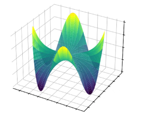
In Figures 3–5 we give the numerical results for the eigenforms, standing waves for the free surface elevation are represented in accordance with the formula above, where $A_n=\{40.53;44.83;48.68\}$ as $n=4,5,6$, respectively. The number of nodes and antinodes is exactly specified by the number $n$.

Figure 3. Eigenform for the elevation as $n=4$.

Figure 4. Eigenform for the elevation as $n=5$.

Figure 5. Eigenform for the elevation as $n=6$.

6. Concluding remarks

1. (i) In this work we have developed a formal asymptotic procedure that enables one to obtain simple approximate formulae for the free surface elevation corresponding to quasimodes of the velocity potential. We have introduced an asymptotic parameter $\gamma a_0$ of the problem which is large provided high-frequency stationary oscillations are studied. The respective solutions exist provided quantisation-type condition (3.17) is valid for the large parameter $\gamma$. This condition contains the geometrical term ${2 V_m}/{\alpha _m}$ that, it seems, cannot be found without asymptotic solution of the problem at hand, e.g. from phenomenological arguments. Having constructed the corresponding quasimodes, we described some of the high-frequency eigenoscillations of the free surface localised near the shoreline of a basin.

   Asymptotic solutions localised near shorelines of water basins were also discussed in Anikin et al. (2019), however, by means of Maslov's canonical operator and for an alternative model. It seems that the most recent asymptotic results on the waves localised near shorelines are discussed in Dobrokhotov, Minenkov & Votiakova (2024) (see also the references therein). The authors make use of the shallow water model and the corresponding equations. The results include formal asymptotics of solutions to the linearised shallow water problem in the form of the localised standing waves. The asymptotic solutions to the corresponding nonlinear problem are then given by means of Carrier–Greenspan transformations.

2. (ii) From the mathematical point of view, in order to assert that the constructed quasimodes and asymptotic formulae for the high frequencies correspond to some actual eigenfunctions and eigenvalues of the operator attributed to the problem (1.5)–(1.7), additional work is required. Such a proof seems to be a difficult task (Lazutkin 1993) and it is not considered herein. It is known from the literature (Babich & Buldyrev 1991) that it was possible to prove that some sequences of actual eigenvalues have the asymptotics coinciding with those constructed on a formal way in the analogous problem for the whispering-gallery modes, Babich & Buldyrev (1991, chapter 7). The analogous results for the eigenfunctions in such a problem are not known to the author.

3. (iii) We have constructed a complex-valued asymptotic solution of the problem for time-harmonic oscillations,

   (6.1)\begin{align} u(s,R,\varphi;\gamma)\mathrm{e}^{-\mathrm{i}\omega t} = \mathrm{e}^{\mathrm{i}[\alpha \gamma s-\omega t]} \{ w_0(s,R,\varphi)+\gamma^{-1}w_1(s,R,\varphi)+ \gamma^{-2}w_2(s,R,\varphi)+\cdots\}. \end{align}
   This solution can be interpreted as a progressive edge wave localised near the shoreline $L$ propagating in the direction of the vector $\boldsymbol {t}(s)={\mathrm {d}\boldsymbol {r}_0(s)}/{\mathrm {d}s}$ with wave velocity ${\mathcal {V}}_{progr}={\omega }/{\alpha \gamma }$. However, considering the real-valued potential $U(x,y,z,t)= \mathrm {Re}\{u(x,y,z)\mathrm {e}^{-\mathrm {i}\omega t}\}$ which actually has the physical meaning as that specifying the velocity of a fluid, $\boldsymbol {V}= \boldsymbol {\nabla } U$, it makes no sense to speak about a progressive wave, see also (5.2). It seems that only the term standing wave has a physical meaning in the theory of linear water edge waves. In this respect, it ought to clarify what is implied by a progressive wave in the linear model that is observed experimentally, for instance, by Huntley et al. (1981).

4. (iv) It is obvious that the nonlinearity and viscosity as well as the surface tension effects cannot be described by the accepted linear model of water waves of small amplitude in this work. Nevertheless, the asymptotic results for the quasimodes of the free surface elevation are given by elementary formulae which can be easily exploited for numerical simulations.