Post-shock turbulence recovery in oblique-shock/turbulent boundary layer interaction flows

Abstract

The oblique shock impinging on the supersonic turbulent boundary layer leads to a mixing layer and the emergence of large-scale coherent structures within the interaction zone which leave significant velocity defect and turbulence amplification downstream. In the present study, we investigate the turbulence recovery in the post-shock region by exploiting direct numerical simulation data of the oblique-shock/turbulent boundary layer interaction flow at the incoming Mach number of $2.28$ and the shock angle of $33.2^\circ$, with special attention paid to the contribution of the mixing layer and large-scale structures to flow dynamics. For that purpose, we propose to split the mean velocity, Reynolds stresses and spanwise spectra into a canonical portion that is constructed according to the statistics of canonical turbulent boundary layers, and a mixing-layer-induced portion. We found that the hidden mixing layer grows with the boundary layer thickness and that the induced mean shear and Reynolds stresses decay at different rates. The mean velocity recovers to the canonical profiles at a distance of 13 boundary layer thicknesses downstream where the mixing-layer-induced mean shear ceases to have strong impacts. The recovery of Reynolds stresses requires 10 boundary layer thicknesses in the near-wall region but a much longer streamwise extent in the outer region due to the slow decay of large-scale motions. These large-scale motions superpose on the near-wall turbulence, intensifying the turbulent fluctuations, yet having a trivial impact on the skin friction, for the contribution of the mixing-layer-induced mean shear and Reynolds shear stress are balanced by the advection term. We further establish a simple physical model capable of approximately predicting the streamwise evolution of mixing-layer-induced mean shear and turbulent kinetic energy. This model suggests that the complete recovery of turbulence in the outer region requires a streamwise extent of approximately 50 boundary layer thicknesses.

1. Introduction

Shock-wave/turbulent boundary layer interaction has been widely investigated due to its significant engineering applications (Delery 1985; Andreopoulos, Agui & Briassulis 2000; Dolling 2001; Smits & Dussauge 2006; Babinsky & Harvey 2011; Gatski & Bonnet 2013). When a supersonic turbulent boundary layer is impinged by an oblique shock wave, the incident and the reflected shock waves lead to pressure rise, mean flow deceleration and even flow separation within the interaction zone due to the low momentum near the wall. The induced abundant flow features have received considerable attention in previous research (Andreopoulos et al. 2000; Dolling 2001; Smits & Dussauge 2006; Babinsky & Harvey 2011; Gaitonde 2015).

Once the flow separation occurs, the mean flow reversal from the separation point to the reattachment point will lead to a strong mixing layer that detaches from the wall. It has been proven by Dupont, Haddad & Debieve (2006), Dupont et al. (2008) and Dupont, Piponniau & Dussauge (2019) that the statistics near this mixing layer resemble those of free mixing layers, including the Reynolds stress, spreading rate and entrainment velocity. Helm, Martín & Williams (2021) further verified this postulation in supersonic/hypersonic turbulent flows over compression ramps at incoming Mach numbers of $3.0$, $7.0$ and $9.0$. The inflectional mean flow profiles lead to Kelvin–Helmholtz instability (Selig et al. 1989; Priebe & Martín 2012), inducing large-scale shedding vortices (Pirozzoli & Grasso 2006; Pirozzoli & Bernardini 2011a; Zhuang et al. 2018). These velocity and pressure fluctuations travel upstream, leading to low-frequency unsteady shock motions and the ‘breathing’ of separation bubbles (Ganapathisubramani, Clemens & Dolling 2007; Wu & Martin 2008; Priebe & Martín 2012; Clemens & Narayanaswamy 2014). They are also convected downstream by the mean flow, resulting in the intensification of wall heat flux and pressure fluctuations (Bernardini, Pirozzoli & Grasso 2011; Volpiani, Bernardini & Larsson 2018, 2020), the enhancement of mass and momentum entrainment between the boundary layer and free-stream flow (Wu & Martin 2007, 2008; Piponniau et al. 2009; Priebe & Martín 2012) and the amplification of the Reynolds stress (Smits & Muck 1987; Zheltovodov, Lebiga & Yakovlev 1989; Fang et al. 2020; Yu et al. 2022).

The flow adjacent to the interaction zone is basically in a non-equilibrium state (Pirozzoli, Bernardini & Grasso 2010; Zuo et al. 2019; Adler & Gaitonde 2020). The statistics and flow structures will take a certain streamwise extent to recover, requiring modifications of turbulent models to capture such non-equilibrium phenomena (Morgan et al. 2013). Therefore, the flow domain under investigation should be sufficiently long in the post-shock region in order to investigate their evolution (Wu & Martin 2007, 2008; Humble, Scarano & van Oudheusden 2009). Previous studies on this recovery process primarily focus on three aspects: mean velocity, turbulent fluctuations and flow structures. In the oblique-shock-wave/turbulent boundary layer interaction (OSBLI) flows, Pirozzoli & Grasso (2006) showed that at the incoming Mach number $M_\infty =2.9$ and the shock angle of $33.2^\circ$, where the flow within the interaction zone goes through mild separation, the mean velocity profile recovers to an equilibrium state at a distance of around 10 boundary layer thicknesses past the interaction zone. During this process, the ‘dip’ in the mean velocity profile, which is the residue of the mixing layer caused by the flow separation within the interaction zone, gradually disappears. For turbulent kinetic energy (TKE) and its transport, the turbulence in the inner region rapidly recovers to the equilibrium state (Pirozzoli & Bernardini 2011a). The relaxation of turbulence in the outer region is incomplete, leaving much stronger turbulent fluctuations even at the end of the computation zone/measuring aera (Pirozzoli & Grasso 2006; Wu & Martin 2007; Baidya et al. 2020). Moreover, the anisotropy and transport of the Reynolds stress tensor resemble those of the free mixing layer (Pirozzoli et al. 2010; Fang et al. 2020). In the aspect of flow structures, recent experimental and numerical investigations have shown that the upstream near-wall small-scale low-speed streaks (Robinson 1991) are twisted as they pass through the interaction zone, and become weaker and less organized right after the reattachment point (Fang et al. 2020). The small-scale near-wall structures recover rapidly within one interaction length scale (Baidya et al. 2020). The large-scale motions, on the other hand, are strengthened by the shock wave and decay slowly downstream, with the wall-normal locations of their maximal intensities statistically aligning with the centre of the mixing layer (Wu & Martin 2008; Humble et al. 2009; Priebe & Martín 2012). Pirozzoli et al. (2010) reported similar phenomena on the previously mentioned three aspects in transonic shock/boundary layer interaction. It is found that the low-speed streaks in the near-wall region are reformed at a distance of five interaction length scales downstream of the impinging shock wave.

The proceeding investigations have revealed that the turbulence upstream and downstream of the interaction zone is disparate, thereby raising the fundamental questions: How do the turbulent structures that are prominent in the post-shock region, such as the mixing layer and the large-scale motions, influence the turbulent dynamics and skin friction? How long will it take for the turbulence to fully recover to the upstream equilibrium state? To answer these questions, we propose to decompose the mean velocity and Reynolds stress into the canonical and mixing-layer-induced portions: the former is constructed as the canonical turbulent boundary layers, leaving the residue as the latter. This decomposition enables us to directly evaluate the contribution of the mixing-layer-related flow features to skin friction and TKE in the post-shock region, thus providing a physical depiction of their evolution and their impact on the flow dynamics. To the best of our knowledge, this method has not been proposed or applied to study OSBLI flows yet.

The remainder of this paper is organized as follows. The physical model and numerical settings are briefly introduced in § 2. The evolution of mean velocity and Reynolds stress downstream of the interaction zone is firstly discussed in § 3. In §§ 4 and 5, the methods to decompose the mean velocity and Reynolds stress are proposed, which are further utilized to investigate the evolution of the mixing-layer-related mean shear and Reynolds stress downstream. Their contributions to the skin friction, TKE and its transport are also discussed. A simplified physical model to roughly predict the turbulent recovery process is proposed in § 6. Concluding remarks are given in § 7.

2. Physical model and numerical implements

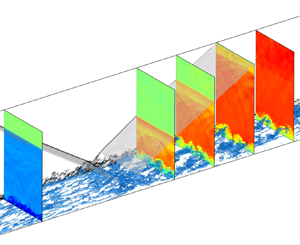
The flow configuration under investigation is depicted in figure 1. We study the fully developed supersonic turbulent boundary layer at the incoming Mach number $M_\infty = 2.28$, temperature $T_\infty = 155.8\,{\rm K}$ and Reynolds number $Re_{in}= \rho _\infty U_\infty \delta _{in} / \mu _\infty =12\,000$, where $\rho _\infty$, $U_\infty$, $\delta _{in}$ and $\mu _\infty$ are the density, velocity, nominal boundary layer thickness (where the mean velocity reaches $99\,\%$ of the free-stream values) and dynamic viscosity of the incoming flow. To simulate the oblique-shock wave generated by a wedge, we impose the inviscid Rankine–Hugoniot (RH) jump condition at the top boundary. The angle of the wedge is set as $8^\circ$, generating an oblique shock impinging at $x_{imp}=30\delta _{in}$ with the angle of $33.2^\circ$. Under these flow parameters, the flow within the interaction zone goes through mild separation (Pirozzoli & Grasso 2006).

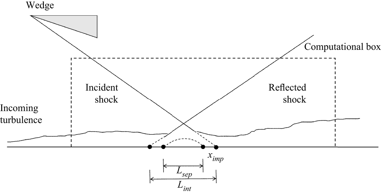
Figure 1. Sketch of the computational domain.

The flow is governed by the following three-dimensional Navier–Stokes equations for a compressible Newtonian gas, satisfying mass, momentum and energy conservations, cast as follows in Cartesian coordinates ($x_i$, $i=1,2,3$, also referred to as $x$, $y$, $z$):

(2.1)$$\begin{gather} \frac{\partial{\rho}}{\partial{t}} + \frac{\partial{\rho u_j}} {\partial{ x_j}}=0 , \end{gather}$$

(2.2)$$\begin{gather}\frac{\partial {\rho u_i}} {\partial {t}} + \frac{\partial {\rho u_i u_j}} {\partial {x_j}}=- \frac{\partial {p}} {\partial {x_i}}+ \frac{\partial{\tau_{ij}}} {\partial {x_j}}, \end{gather}$$

(2.3)$$\begin{gather}\frac{\partial{\rho E}}{\partial{t}}+\frac{\partial{\rho u_j E}}{\partial{x_j}}=-\frac{\partial{p u_j}}{\partial{x_j}}+ \frac{\partial{u_i \tau_{ij}}} {\partial {x_j}} - \frac{\partial{q_j}} {\partial{x_j}}, \end{gather}$$

where $\rho$, $p$ and $T$ represent density, pressure and temperature and $u_i$ ($i=1,2,3$, also referred to as $u$, $v$, $w$) the velocity in $x_i$ direction. The thermodynamic quantities satisfy the state equations for the calorically perfect gas

(2.4a–c)\begin{equation} p=\rho R T,\quad E = e + \tfrac{1}{2}u_i u_i,\quad e=C_v T. \end{equation}

The viscous stress and heat transfer are obtained by the constitutive equations for Newtonian gas, i.e.

(2.5a,b)\begin{equation} \tau_{ij}=2\mu S_{ij}-\frac{2}{3}\mu S_{kk} \delta_{ij},\quad q_j=- \lambda \frac{\partial{T}}{\partial{x_j}}, \end{equation}

with $S_{ij}$ the strain rate tensor. The dynamic viscosity $\mu$ is determined by Sutherland's law and heat conductivity $\lambda =\mu /(Pr C_p)$, with the Prandtl number is set as $Pr=0.72$. The gas constant, constant-pressure and constant-volume specific heat are denoted by $R$, $C_p$ and $C_v$, respectively.

The boundary conditions are specified as follows. The mean velocity of the incoming turbulent boundary layer is given by the formula proposed by Musker (1979). The velocity fluctuations are generated by the synthetic digital filtering approach as in Klein, Sadiki & Janicka (2003). The average and fluctuation of temperature are determined by those of the velocity with the generalized Reynolds analogy (Zhang et al. 2014). The non-reflecting conditions proposed by Pirozzoli & Colonius (2013) are adopted at the top and outflow boundaries, except that the inviscid RH jump condition is enforced at the top boundary, as stated previously. At the lower wall, no-slip and no-penetration conditions are applied for velocity, and the isothermal condition is applied for temperature, set as $T_w=1.92 T_\infty$, the recovery temperature of the incoming flow, to mimic an adiabatic wall. Periodic conditions are applied in the spanwise direction.

Direct numerical simulation (DNS) is performed utilizing the open-source ‘STREAmS’ solver developed by Bernardini et al. (2021), which solves the governing equations (2.1)–(2.5a,b) by the finite difference method. This solver has been widely verified in supersonic channels, boundary layers and OSBLI flows. The convective terms are approximated by the sixth-order kinetic-energy-preserving scheme (Pirozzoli 2010), and switched to the fifth-order weighted essentially non-oscillation scheme (Jiang & Shu 1996) when strongly compressive events are detected by the criterion used in Ducros et al. (1999). The viscous terms are cast as Laplacian forms and approximated by the sixth-order central difference scheme. Wray's three-stage third-order scheme is adopted for time advancement (Wray 1990).

The sizes of the computational domain in the streamwise ($x$), wall-normal ($y$) and spanwise ($z$) directions are set as $60 \delta _{in}$, $12 \delta _{in}$ and $6.5 \delta _{in}$, respectively. It is discretized by $2000 \times 320 \times 240$ grids in the three directions. The grids are uniformly distributed in the $x$ and $z$ directions with the mesh intervals being ${\rm \Delta} x^+ \approx 5.4$ and ${\rm \Delta} z^+ \approx 4.9$ under viscous scales at the inlet of the boundary layer. In the wall-normal direction, the grids are stretched by a hyperbolic-sine function within $y=2.5\delta _{in}$ and uniformly distributed above it. The minimal grid interval is set at the wall, being ${\rm \Delta} y^+_w \approx 0.7$.

The statistics are averaged in the spanwise direction with 900 instantaneous flow fields over the period of $t=351 \delta _{in} / U_\infty \sim 959 \delta _{in} / U_\infty$. To further obtain smoother statistics, the results are also averaged in the streamwise direction across 11 grids, within which the streamwise variation of the mean flow is insignificant. The database has been validated in our previous study (Yu et al. 2022), including the streamwise distributions of the skin friction and mean pressure and the wall-normal distributions of the mean velocity and Reynolds stresses upstream of the interaction zone. The reference station free from the impact of the impinging shock wave is chosen at $x_r = 15.0 \delta _{in}$. Some of the important flow parameters at this station are listed in table 1, denoted by the subscript $r$. The mean velocity and turbulent fluctuations upstream of the interaction zone, the skin friction and wall pressure distributions along the streamwise direction agree with the reference in Bernardini et al. (2016). In discussing those results, we reported that the lengths of the interaction and separation zones are $L_{int} \approx 3.27 \delta _r$ and $L_{sep} \approx 1.65 \delta _r$, respectively, consistent with the results reported by Volpiani et al. (2018, figure 12).

Table 1. Statistics at the reference plane $x_r=15.0 \delta _{in}$. Here, the skin friction coefficient is defined as $C_f = 2 \tau _w / (\rho _\infty U^2_\infty )$, $\delta ^*_r$ and $\theta _r$ are the displacement and momentum thicknesses, $Re_{\theta r} = \rho _\infty U_\infty \theta _r / \mu _\infty$, friction Reynolds number $Re_{\tau r} = \rho _w u_\tau \theta _r / \mu _w$ and shape factor $H_r = \delta ^*_r / \theta _r$.

As further validation of the velocity variances in the post-shock region, in figure 2, we compare the distributions of the non-zero Reynolds stress components with those reported by Bernardini et al. (2016). The Reynolds stress normalized by the mean kinetic energy of the incoming free-stream flow is defined as

(2.6)\begin{equation} R_{u_i u_j} = \frac{\overline{\rho u''_i u''_j}}{\rho_\infty U^2_\infty}. \end{equation}

Herein, the ensemble average of a generic flow quantity $\varphi$ is denoted as $\bar \varphi$, and the corresponding fluctuation by $\varphi '$, the density-weighted average (or Favre average) by $\tilde \varphi$ and the corresponding fluctuation $\varphi ''$. The superscript $*$ denotes the rescaled interaction coordinate, defined as

(2.7a,b)\begin{equation} x^* = (x-x_{imp})/\delta_r,\quad y^* = y/\delta_r. \end{equation}

Figure 2. Reynolds stress distribution, (a) $R_{uu}$, (b) $R_{vv}$, (c) $R_{ww}$, (d) $R_{uv}$, flooded: present results, lines: reference data from Bernardini et al. (2016).

Quantitatively, the results in the present study conform reasonably well with those in Bernardini et al. (2016). The slight difference can be attributed to the different Reynolds numbers between the two datasets. They are also qualitatively consistent with the results reported by previous studies (Pirozzoli & Bernardini 2011a; Bernardini et al. 2016; Fang et al. 2020). Upstream of the interaction zone ($x^* \lesssim -3.0$), the maxima of the Reynolds normal and shear stresses are attained in the near-wall region below $y^* \approx 0.1$. As the flow goes through the interaction zone, the normal components of the Reynolds stress (figure 2a–c) are greatly amplified, with their peaks rising from the near-wall region to $y^* \approx 0.3$. It has been proven in our previous study (Yu et al. 2022) that the physical counterparts of the highly intensified turbulent fluctuations in the outer region are the large-scale low-speed streaks and cross-stream circulations downstream of the interaction zone, as can be visualized in figure 3. As the flow approaches further downstream, the large-scale structures gradually decay. The instantaneous field in figure 3(a) and the reappearing near-wall peak of $R_{uu}$ below $y^* \approx 0.1$ in figure 2(a) further indicate that the near-wall small-scale structures start to reform at $x^* \approx 4.0$. The Reynolds shear stress in figure 2(d) reaches maxima at $x^* \approx 1.0$, a slightly downstream location compared with the Reynolds normal stresses.

Figure 3. Instantaneous fields, isosurface of (a) velocity fluctuation $u''/U_\infty =-0.1$, (b) the second invariant of velocity gradient $Q=10.0$, coloured by the wall-normal coordinate $y$. Transparent isosurfaces: incident and reflected shocks, vertical slices: numerical Schlieren $\exp (-|\boldsymbol {\nabla } \rho |/\rho )$.

3. Mean velocity and Reynolds stress

In the subsequent discussions, we primarily present the statistical results at the streamwise station $x_r= 15 \delta _{in}$ ($x^*_r=-10.0$) as the reference for canonical wall-bounded turbulence, and at the stations downstream the interaction zone at $x_1=35 \delta _{in}$ ($x^*_1 = 3.3$), $x_2=40 \delta _{in}$ ($x^*_2 = 6.7$), $x_3=45 \delta _{in}$ ($x^*_3 = 10.0$), $x_4=50 \delta _{in}$ ($x^*_4 = 13.3$) and $x_5=55 \delta _{in}$ ($x^*_5 = 16.7$) to analyse the turbulent evolution in the post-shock region, as displayed in figure 4. Line legends are listed in table 2.

Figure 4. Streamwise stations in the subsequent analysis. Contours on the cross-stream slices: velocity fluctuation $u''/U_\infty$, on the vertical slice: numerical Schlieren $\exp (-|\boldsymbol {\nabla } \rho |/\rho )$.

Table 2. Streamwise stations and line legends in the subsequent analysis.

The mean velocity profiles at the six streamwise stations are displayed in figure 5. The abscissa and the ordinate in figure 5(a) are normalized by the local boundary layer thickness $\delta$ and the mean velocity at the outer edge of the boundary layer $u_\delta$, hereinafter referred to as the ‘outer scales’. Figure 5(b) displays the van Driest transformation of mean velocity, written as

(3.1)\begin{equation} u^+_{VD} = \frac{1}{u_\tau} \int^{\tilde u}_0 \sqrt{\frac{\bar \rho}{\bar \rho_w}}\, {\rm d} u. \end{equation}

The abscissa and the ordinate are normalized by viscous scales, defined as

(3.2a–d)\begin{equation} \tau_w = \mu_w \left.\frac{\partial \bar u}{\partial y}\right|_w,\quad u_\tau = \sqrt{\frac{\tau_w}{\bar \rho_w}},\quad \delta_\nu = \frac{\mu_w}{\bar \rho_w u_\tau},\quad y^+= \frac{y}{\delta_\nu}, \end{equation}

with $\tau _w$, $\bar \rho _w$ and $\mu _w$ denoting the mean shear stress, density and dynamic viscosity on the wall. The van Driest transformed velocity at the reference station $x_r$ follows that of the canonical wall-bounded turbulence, obeying the linear law in the viscous sublayer $y^+ \lesssim 5$, and the logarithmic law above $y^+ \approx 30$. For the mean velocity at $x_1$ immediately downstream of the interaction zone, the intercept in the logarithmic region is significantly lower than the standard value $5.0$, while the velocity in the wake region rises to a higher value. This indicates a lower wall shear stress and a stronger mean shear above $y^+ \approx 10$. Under the outer scales, it is observed that the velocity defect is increased, and there is an obvious inflection point at $y/\delta \approx 0.3$. These are caused by the mixing layer related to the flow retardation and separation within the interaction zone. Compared with the mean velocity profile at $x_r$, the shear rate is lower below $y/\delta \approx 0.1$, and much higher from $y /\delta \approx 0.2$ to the outer edge of the boundary layer. As it goes downstream, the mean velocity profiles gradually return to those of the canonical wall-bounded turbulence. At $x_4$, a distance nearly $13.3 \delta _r$ downstream of the impinging point, the intercepts in the logarithmic region rise anew to $5.0$ and the residue of the mixing layer vanishes visually. These results are consistent with those reported in previous studies (Pirozzoli & Grasso 2006; Baidya et al. 2020).

Figure 5. Mean velocity profiles, (a) normalized by outer scales, (b) van Driest transformed, normalized by viscous scales. Line legends refer to table 2, symbols: reference data reported by Pirozzoli & Bernardini (2011b) at $M_\infty =2$ and $Re_\tau =200$.

The Reynolds stress distributions have been discussed in § 2. Here, we primarily focus on the distributions of Reynolds stress components along the wall-normal direction at the six streamwise stations in figure 4 and table 2. The results are plotted under viscous scales in figure 6. Compared with the statistics at the reference station $x_r$, all the Reynolds stress components are enhanced, especially in the outer region. As it approaches downstream, the peaks in the outer region gradually diminish. These peaks retain significant until the end of the computational zone, suggesting that the decay of these large-scale motions requires a streamwise extent much longer than $16.7 \delta _r$.

Figure 6. Wall-normal distributions of Reynolds stresses, normalized by the wall shear stress $\tau _w$, (a) $R^+_{uu}$, (b) $R^+_{vv}$, (c) $R^+_{ww}$ and (d) $-R^+_{uv}$. Symbols: reference data at $Re_\tau \approx 200$ and $M_\infty =2$ (Pirozzoli & Bernardini 2011b). Line legends refer to table 2.

In the inner region within $y^+ \lesssim 30$, $R^+_{vv}$ and $-R^+_{uv}$ downstream $x^*_3 =10$ collapse to those at $x_r$. These are reckoned as the ‘detached variables’ in the concept of the ‘attached-eddy model’ (Townsend 1976; Hwang 2015). The large-scale motions in the outer region do not leave strong ‘footprints’ in the near-wall region due to the no-penetration condition. Parameters $R^+_{uu}$ and $R^+_{ww}$, on the other hand, are the wall-attached variables and do not share such a feature. The value of $R^+_{uu}$ collapses to a uniform distribution below $y^+ \approx 40$ downstream of $x_2$ but obviously higher than the statistics at the reference station $x_r$. The value of $R^+_{ww}$ continuously decreases with $x$, whose convergence is not achieved until $x_5$. We attribute these seemingly anomalous behaviours to two contradictory factors: the increasing Reynolds number and the decaying large-scale motions in the outer region. The increasing Reynolds number intensifies wall-attached velocities in the near-wall turbulence (Cheng et al. 2020; Smits 2020; Chen & Sreenivasan 2021). The large-scale motions in the outer region leave footprints on the near-wall region, enhancing the near-wall turbulent intensities (Marusic, Mathis & Hutchins 2010; Mathis, Hutchins & Marusic 2011). In turn, the decay of those large-scale motions will lead to the diminishment of the near-wall fluctuation variances. Based on this scenario, we conjecture that, for the $R^+_{uu}$ component, the two factors are coincidentally cancelled out, leading to the convergence of the near-wall fluctuation variances. As for the $R^+_{ww}$ component, the decaying of the large-scale motions has more influence on the near-wall turbulence than the increasing Reynolds number, thereby continuously decreasing the near-wall fluctuation intensity as the flow approaches downstream. This statement will be further supported by the discussions in § 5.1.

Considering that the $R^+_{uu}$ and $R^+_{ww}$ components are highly affected by the Reynolds number and the large-scale motions in the outer region that decay particularly slowly, we suggest to determine the recovery of the near-wall turbulence by either $R^+_{vv}$ or $-R^+_{uv}$. Therefore, the near-wall turbulence is concluded to return to the canonical and equilibrium state at $x^*_3 = 10.0$.

4. Skin friction contributed by the mixing layer

4.1. Extracting the mixing layer

The qualitative descriptions of the mean velocity profiles in figure 5 revealed that the mixing layer due to the flow separation within the interaction zone is retained downstream. In other words, there exists a mixing layer hidden inside the boundary layer. To quantitatively depict its distribution, we propose to construct the mean velocity profile as in the canonical wall-bounded turbulence, denoted by $\tilde u_c$, thereby the mixing-layer-induced portion $\tilde u_m$ can be obtained as $\tilde u_m = \tilde u_c - \tilde u$ to ensure it is positive. The van Driest transformed canonical mean profile is constructed as follows:

(4.1)\begin{align} \tilde u^+_{c,VD}=\left\{\begin{array}{@{}ll} \tilde u^+_{r,VD}(y^+), & y^+<30 \\ 2.55 \ln{y^+}+5, & y^+>30, y/\delta<0.3 \\ 2.55 \ln{y^+}+5+2.55 \beta (\cos(0.3{\rm \pi})- \cos({\rm \pi} y/\delta)), & 0.3 < y/\delta <1 \\ 2.55 \ln{\delta^+}+5+2.55 \beta (\cos(0.3{\rm \pi})+1), & y/\delta>1. \\ \end{array}\right. \end{align}

In this formula, the mean velocity within the buffer layer $y^+<30$ is interpolated from that at the reference station $x_r$. In the logarithmic region between $y^+>30$ and $y/\delta < 0.3$, it is constructed by the standard logarithmic law of the turbulent boundary layer (Pirozzoli & Bernardini 2011b). In the outer region $0.3 < y/\delta <1.0$, the wake law is further added. Considering that the friction Reynolds number is relatively low and varying in the streamwise direction, the coefficient $\beta$ differs at different streamwise locations. Postulating that the variation of $\beta$ with $Re_\tau$ is linear and that the recovery of the mean velocity is achieved at $x_5$, this function can be expressed as $\beta =0.0005 Re_\tau - 0.411$, with the coefficients obtained from the mean profiles at $x_r$ and $x_5$. The reversed van Driest transformation is further adopted to obtain the $\tilde u_c$ distribution.

The original and the constructed canonical mean velocity profiles are shown in figure 7(a,b), normalized by viscous and outer scales, respectively. The constructed canonical mean velocity distributions $\tilde u_c$ by formula (4.1) conform with those at $x_r$, $x_4$ and $x_5$, indicating its validity. The divergence of the original mean velocity profiles $\tilde u$ from the canonical profiles $\tilde u_c$ gradually weakens as it approaches downstream. This ‘gap’ is the mixing-layer-induced portion $\tilde u_m$, whose distribution is shown in figure 7(c). In the wall-normal direction, $\tilde u_m$ attains maximum at $y=0.2\delta$. Above this location until the outer edge of the boundary layer, $\tilde u_m$ decreases monotonically. This mixing layer grows with the boundary layer, with the identical thicknesses. At $x_4$ and $x_5$, this mixing layer ceases to have strong impact on the mean flow, with its contribution to the mean velocity by less than $4\,\%$. The mean gradient of $\tilde u_m$ across the boundary layer is shown in figure 7(d) with symbols. Cubic polynomials are adopted to fit the curves, in order to locate the approximate maxima. As marked with the solid symbols in figure 7(c,d), the maximal velocity gradient lies at $y/\delta \approx 0.65$ and is weakly dependent on the streamwise location. According to our examination, the self-similarity of the mean profiles can be roughly satisfied when normalized by their maxima. However, due to the restriction of the lower wall, the distribution of mean velocity and its gradient are unsymmetrical.

Figure 7. Mean velocity distributions, (a,b) original $\tilde u$ and constructed $\tilde u_c$, (a) van Driest transformation normalized by viscous scales, (b) normalized by outer scales, lines with symbols: $\tilde u$, lines: $\tilde u_c$. (c) Mixing-layer-induced portion $\tilde u_m$. (d) Open symbols: gradient of $\tilde u_m$, lines: curve fitting with cubic polynomials within $y/\delta = 0.3 \sim 0.9$, solid symbols: the maxima of the fitting curve. Line legends refer to table 2.

4.2. Splitting the Reynolds shear stress and skin friction

We further extract the Reynolds shear stress induced by the mixing layer in the post-shock region. To do this, we propose to split the total shear stress $\bar \tau$ as follows:

(4.2)\begin{align} \bar \tau & = \bar \tau_v + \bar \tau_t \nonumber\\ &= \bar \tau_{v,c} + \bar \tau_{v,m} + \bar \tau_{t,c} + \bar \tau_{t,m} \nonumber\\ &= \bar \tau_{c} + \bar \tau_{v,m} + \bar \tau_{t,m}, \end{align}

with $\bar \tau _v$ and $\bar \tau _t$ denoting the viscous and Reynolds shear stresses, and the subscripts $c$ and $m$ the constructed canonical and the mixing-layer-induced portions, respectively. The mixing-layer-induced Reynolds shear stress $\bar \tau _{t,m}$ is therefore obtained as

(4.3)\begin{equation} \bar \tau_{t,m} = \bar \tau - \bar \tau_c - \bar \tau_{v,m}, \end{equation}

under the assumption that the $\bar \tau _c$ values at each location are the same function of $y/\delta$ as that of $x_r$ due to the self-similarity of turbulent boundary layers over flat walls (Kumar & Mahesh 2021). The original Reynolds shear stress $\bar \tau _t$ and its canonical portion $\bar \tau _{t,c}$ are plotted in figure 8(a,b). The latter collapse well at different streamwise stations, except for the slight difference below $y=0.1\delta$. The mixing-layer-induced portion $\bar \tau _{t,m}$ displayed in figure 8(c) decreases monotonically as it approaches downstream. The maximal values are attained approximately at the same wall-normal locations $y/\delta \approx 0.5$, lower than those of the maximal gradient of $\tilde u_m$.

Figure 8. Distributions of Reynolds shear stress in the wall-normal direction, (a) original $\bar \tau _t$, (b) constructed canonical portion $\bar \tau _{t,c}$, (c) mixing-layer-induced portion $\bar \tau _{t,m}$. Line legends refer to table 2.

The skin friction contributed by the mixing-layer-induced mean shear and Reynolds shear stress is evaluated utilizing the decomposition formula proposed by Renard & Deck (2016) (hereinafter referred to as the ‘RD formula’). This formula was extended to compressible turbulent boundary layers by Fan, Li & Pirozzoli (2019), written as

(4.4)\begin{align} C_f &= \underbrace{\frac{2}{\rho_\delta u^3_\delta} \int^\delta_0 \bar \tau_{v,xy} \frac{\partial \tilde u}{\partial y} {\rm d}y}_{C_V} +\underbrace{\frac{2}{\rho_\delta u^3_\delta} \int^\delta_0 \bar \tau_{t,xy} \frac{\partial \tilde u}{\partial y} {\rm d}y}_{C_T} +\underbrace{\frac{2}{\rho_\delta u^3_\delta} \int^\delta_0 (\tilde u - u_\delta) \frac{\partial \bar p}{\partial x} {\rm d}y}_{C_P} \nonumber\\ &\quad + \underbrace{\frac{2}{\rho_\delta u^3_\delta} \int^\delta_0 (\tilde u - u_\delta) \left(\bar \rho \left(\tilde u \frac{\partial \tilde u}{\partial x} + \tilde v \frac{\partial \tilde u}{\partial y}\right) -\frac{\partial}{\partial x} (\bar \tau_{v,xx}+\bar \tau_{t,xx})\right) {\rm d}y}_{C_G}, \end{align}

where $C_V$, $C_T$ and $C_G$ denote the skin friction caused by viscous shear stress, Reynolds shear stress and mean advection, respectively. The mean pressure-gradient term, $C_P$, is only significant within the interaction zone, as will be demonstrated later. Divided by the skin friction coefficient $C_f$, these terms can be formulated as

(4.5)$$\begin{gather} \frac{C_V}{C_f}=\int^{\delta^+}_0 \frac{u_\tau}{u_\delta} \bar \tau^+_{v,xy} \frac{\partial \tilde u^+}{\partial y^+} {\rm d}y^+ \end{gather}$$

(4.6)$$\begin{gather}\frac{C_T}{C_f}= \int^{\delta^+}_0 \frac{u_\tau}{u_\delta} \bar \tau^+_{t,xy} \frac{\partial \tilde u^+}{\partial y^+} {\rm d}y^+ \end{gather}$$

(4.7)$$\begin{gather}\frac{C_G}{C_f}= \int^{\delta^+}_0 \left( \frac{\tilde u}{u_\delta} -1 \right) \frac{\partial \bar \tau^+_{xy}}{\partial y^+} {\rm d}y^+. \end{gather}$$

We further substitute the proposed decomposition for the mean velocity and the Reynolds shear stress, i.e. $\tilde u = \tilde u_c - \tilde u_m$ and $\bar \tau _t = \bar \tau _{t,c} + \bar \tau _{t,m}$, into the first two terms $C_V$ and $C_T$, they can further be decomposed as those contributed genuinely by the canonical portions and the mixing-layer-related portions,

(4.8a,b)$$\begin{gather} \frac{C_{Vc}}{C_f}= \int^{\delta^+}_0 \frac{u_\tau}{u_\delta} \bar \tau^+_{v,xy,c} \frac{\partial \tilde u^+_c}{\partial y^+} {{\rm d}y}^+,\quad \frac{C_{Vm}}{C_f}=\frac{C_{V}}{C_f}-\frac{C_{Vc}}{C_f}. \end{gather}$$

(4.9a,b)$$\begin{gather}\frac{C_{Tc}}{C_f}= \int^{\delta^+}_0 \frac{u_\tau}{u_\delta} \bar \tau^+_{t,xy,c} \frac{\partial \tilde u^+_c}{\partial y^+} {{\rm d}y}^+,\quad \frac{C_{Tm}}{C_f}=\frac{C_{T}}{C_f}-\frac{C_{Tc}}{C_f}. \end{gather}$$

The pre-multiplied integrands of these terms (denoted by the subscript ‘$int$’) in the wall-normal direction are displayed in figure 9. Compared with the distributions at the upstream reference station $x_r$, the magnitudes of the viscous term $C_V$ (figure 9a) are lower below $y^+ \approx 30$ in the near-wall region at $x_1$, $x_2$ and $x_3$ downstream of the interaction zone. This can be easily inferred from the mean velocity profiles. The mean shear related to the mixing layer is of the opposite sign to that of the canonical mean velocity, leading to the lower total mean shear. Its canonical portion $C_{Vc}$ (figure 9b) is higher in the post-shock region, which is compensated by the negative mixing-layer-induced portion $C_{Vm}$ (figure 9c). Although the mean shear in the outer region is much stronger than the canonical profile from $x_1$ to $x_3$ (recall figure 7), the pre-multiplied integrand is small, indicating its negligible integrated contribution to the skin friction.

Figure 9. Distribution of the pre-multiplied integrands in formulas (4.4)- (4.9a,b), normalized by viscous scales. (a–c) Viscous terms, (a) $C_{V,int}$, (b) $C_{Vc,int}$, (c) $C_{Vm,int}$. (d–f) Reynolds shear stress terms, (d) $C_{T,int}$, (e) $C_{Tc,int}$, (f) $C_{Tm,int}$. (g) Advection term $C_{G,int}$. Line legends refer to table 2.

The pre-multiplied integrands of the Reynolds stress term $C_T$ (figure 9d) increase significantly in the outer region, while those in the inner region remain almost unaffected compared with that of the upstream reference station at $x_r$. We can infer from figure 9(e) that the unchanged part is primarily attributed to the canonical portion $C_{Tc}$, whose variation in the outer region is also not prominent against the streamwise location. The mixing-layer-induced portion $C_{Tm}$ (figure 9f), on the other hand, contributes significantly to the skin friction in the outer region.

The pre-multiplied integrands of the advection term $C_G$, as shown in figure 9(g), are negligible below $y^+ = 10$. They first decrease to a negative value, then increase and alter their signs in the outer region. The areas surrounded by the abscissa and the negative part of the curve are greater than the positive part, resulting in their negative overall contributions to the skin friction.

The decomposed skin friction terms in formulas (4.4)–(4.9a,b) along the streamwise direction are reported in figure 10. The summation $(C_V+C_T+C_G)/C_f$ is higher than 0.997, indicating that the presently used RD formula for zero-pressure-gradient boundary layers is valid when discussing the skin friction upstream and downstream of the interaction zone. The mean pressure gradient outside the interaction zone is not high enough to manifest their magnitude. Upstream of the interaction zone, the viscous term $C_V$ and the Reynolds shear stress term $C_T$ constitute the total skin friction $C_f$ almost equivalently by around $50\,\%$, while the advection term $C_G$ by less than $10\,\%$. As the flow approaches the shock wave, the advection term $C_G$ decreases to a negative value, while the $C_V$ and $C_T$ terms increase. Due to the flow separation, the total skin friction within the interaction zone (grey-shaded region) is small, and therefore will not be discussed here. Downstream of the interaction zone, the viscous term $C_V$ constitutes the skin friction by around $40\,\%$. The constructed canonical portion $C_{Vc}$ is almost the same as $C_V$, as it can be inferred from figure 9(a,b). The Reynolds shear stress term $C_T$ is significantly higher than the viscous term $C_V$, even higher than the skin friction $C_f$ itself. Its canonical portion $C_{Tc}$, however, contributes to the skin friction by around $50\,\%$, similar to the upstream $C_T$ term. This high ratio primarily comes from its mixing-layer-induced term $C_{Tm}$, which is mostly balanced by the negative $C_G$ term. To verify this statement, we also report the summation of the mixing-layer-induced terms and the advection term, i.e. $C_{Vm} + C_{Tm} + C_G$ in figure 10. Their overall contribution to the total skin friction is less than $15\,\%$, and this percentage decreases to around $11\,\%$ at $x^* \approx 10.0$ and retains this value further downstream. We may conclude that although the mixing-layer-induced large-scale motions in the outer region are significant (recall figure 6), its contribution to the skin friction is trivial.

Figure 10. Skin friction decomposition by the RD formula in (4.4)–(4.9a,b), grey-shaded region: interaction zone, with the extension of $1.2 \delta _r$ in both directions.

In the aspect of its physical significance, the RD formula is obtained by integrating the mean kinetic energy (MKE) budget in the convective frame (Renard & Deck 2016). The physical interpretations of $C_V$, $C_T$ and $C_G$ terms are quite straightforward, representing the mean power supplied by the wall that transfers the MKE to (a) internal energy by viscous dissipation ($C_V$ term), (b) TKE by turbulent production ($C_T$ term) and (c) spatial growth of the boundary layer ($C_G$ term). It can be proved that $C_G$ should satisfy $0 \leq C_G/C_f \leq 1$ under the assumption that the TKE production is non-negative and the total shear stress is non-increasing. The former can be satisfied in the presently studied flow (see figure 15 below). The latter, however, cannot be guaranteed, as it can be inferred from the Reynolds shear stress distributions in figure 8. The negativity of $C_G$ term indicates that the loss of MKE in the convective frame, or the entrainment of MKE from the mean flow in the wall frame (Renard & Deck 2016). The following equation may provide further interpretation:

(4.10)\begin{equation} \tfrac{1}{2} \rho \tilde u^3_\delta \left( \delta^* + \delta^{**} \right) = \tfrac{1}{2} \left( \rho \tilde u^3_\delta \delta - \int^\delta_0 \rho \tilde u^3 \,{\rm d}y \right), \end{equation}

with $\delta ^*$ and $\delta ^{**}$ denoting the displacement and kinetic energy thicknesses. The summation $(\delta ^* + \delta ^{**})$ reflects the loss of kinetic energy in the boundary layer. As shown in figure 11, although the nominal boundary layer thickness $\delta$ grows rapidly downstream of the interaction zone, the displacement and kinetic energy thicknesses almost remain constants, suggesting that the MKE is merely redistributed along the wall-normal direction by mean convection without significant dissipation.

Figure 11. Evolution of boundary layer thicknesses, (a) nominal boundary layer thickness $\delta / \delta _r$, (b) red dashed line: displacement thickness $\delta ^*/ \delta _r$, blue dash-dotted line: kinetic energy thickness $\delta ^{**} /\delta _r$, black solid line: $(\delta ^*+\delta ^{**})/\delta _r$.

In this section, we propose to decompose the mean velocity and the Reynolds shear stress in the post-shock region as the canonical and the mixing-layer-induced portions to investigate the mixing layer hidden inside the boundary layer. Its contribution to skin friction is further evaluated utilizing the skin friction decomposition formula proposed by Renard & Deck (2016) and Fan et al. (2019). Although the mean shear and the Reynolds shear stress related to the mixing layer are strong, they only constitute a small portion of the total skin friction, which is primarily composed of the canonical viscous and Reynolds stress components $C_{Vc}$ and $C_{Tc}$.

5. Turbulent kinetic energy

5.1. Splitting the kinetic energy

Unlike the mean velocity and the Reynolds shear stress, the decomposition of velocity fluctuation variances into its canonical and mixing-layer-induced portions is no simple task. Despite the recent progress made by Chen & Sreenivasan (2021), Smits et al. (2021) and Smits & Hultmark (2021), it is still challenging to construct the canonical portion directly. Therefore, we adopt a different strategy, to follow the ‘inner–outer decomposition’ proposed by Hu & Zheng (2018) and Wang, Hu & Zheng (2021). In their studies, the empirical functions of the near-wall spectra that are considered to be Reynolds number independent are formulated utilizing the results of a turbulent channel flow at $Re_\tau = 110$, thereby decomposing the spectra and variances of velocity fluctuation into the inner and outer portions. Instead of seeking for such empirical functions, in the present study, we simply reckon the spanwise spectra at the reference station $x_r$ as the canonical near-wall portion $E_{u_i u_i,c}$. The mixing-layer-induced portion $E_{u_i u_i,m}$ is thus obtained by subtraction. Integrating the spectra over the wavenumber $k_z$, we may further obtain their fluctuation variances. Note that all the above-mentioned procedures are completed under viscous scalings.

The pre-multiplied spanwise spectra of the density-weighted velocity fluctuations $\sqrt {\rho } u''_i$ at $x_3$ are shown in figure 12. We first discuss their canonical portions, namely the spectra at $x_r$, as displayed in figure 12(a–c). Expectedly, the distributions of these spectra resemble those of the low Reynolds number canonical wall-bounded turbulence (Hwang 2013; Yin, Huang & Xu 2017; Wang, Wang & He 2018). For the streamwise component, the spectra $k_z E^+_{uu}$ attain maxima at $y^+ \approx 12$ with the characteristic length scale of $\lambda ^+_z \approx 100$, representing the near-wall low-speed streaks. The peaks of the spectra of the wall-normal and spanwise components $k_z E^+_{vv}$ and $k_z E^+_{ww}$ are reached at $y^+ \approx 50$ and $y^+ \approx 20$, respectively, with the characteristic length scale of $\lambda ^+_z \approx 150$, representing the quasi-streamwise vortices in the near-wall region.

Figure 12. Pre-multiplied spanwise spectra for density-weighted velocity fluctuations at $x_3$, (a–c) canonical portion $k_z E^+_{u_i u_i,c}$, normalized by viscous scales, (d–f) the original spectra, $k_z E_{u_i u_i}$, (g–i) the mixing-layer-induced portion, $k_z E_{u_i u_i,m}$, normalized by outer scales, (a,d,g) streamwise component $k_z E_{uu}$, (b,e,h) wall-normal component $k_z E_{vv}$, (c,f,i) spanwise component $k_z E_{ww}$.

The pre-multiplied spanwise spectra at $x_3$ for the three velocity components are shown in figure 12(d–f). For the streamwise component, there are two peaks in the $k_z E_{uu}$ distribution, representing the small-scale low-speed streaks in the near-wall region and the large-scale motions in the outer region. The latter lies at $y^* \approx 0.5$ with the characteristic scale of $\lambda ^*_z \approx 1.0$. The spectra of the other two components $k_z E_{vv}$ and $k_z E_{ww}$ do not manifest the double-peak feature, while they spread more widely in the scale space compared with the canonical near-wall spectra in figure 12(b,c). The peaks are also located in the outer region at $y^* \approx 0.5$ with the characteristic scale of $\lambda ^*_z \approx 1.0$, the same as those of the $k_z E_{uu}$ distribution.

The mixing-layer-induced portions, with the canonical near-wall spectra removed, are shown in figure 12(g–i). For the streamwise component $k_z E_{uu,m}$, the peak in the inner region at small scales is substituted by a small-valued negative region. The same phenomenon has been observed by Hu & Zheng (2018), which was explained to be caused by the nonlinear modulation effect of the large-scale motions on the small-scale motions. The peak of the spectra in the outer region retains, penetrating to the near-wall region and leaving ‘footprints’, similar to the ‘superposition effect’ of the large-scale structures in high Reynolds number wall-bounded turbulence (Marusic et al. 2010; Mathis et al. 2011; Smits 2020). This leads to the increment of the turbulent intensities in the inner region, further supporting our previous discussions in § 3. The wall-normal velocity is not a wall-attached variable, therefore the large-scale motions corresponding to the peak in the outer region of the spectra $k_z E_{vv,m}$ have no obvious superposition effect on the near-wall turbulence. The spectra of the spanwise component $k_z E_{ww,m}$ resemble those of the streamwise component $k_z E_{uu,m}$, except that the superposition effects are stronger and spread wider in scale space. This is consistent with our previous presumption in § 3 that the superposition effect has more impact on the near-wall spanwise velocity intensity.

The spectra at the other streamwise locations $x_1$, $x_2$, $x_4$ and $x_5$ (not shown here) are similar to those at $x_3$, with the approximately identical wall-normal locations and spanwise length scales of the peaks in the outer region. This partially reflects the self-similarity of these mixing-layer-induced large-scale motions.

Integrating the mixing-layer-induced spectra, we can further obtain the corresponding velocity fluctuation variances (Reynolds normal stress components). The results are shown in figure 13, where the Reynolds shear stress is also plotted for comparison (note that the Reynolds shear stress plotted here is also obtained via the ‘spectrum removal’ procedure in this section for the consistency of discussion). Expectedly, the turbulent fluctuation intensities decrease as the flow approaches downstream. At $x_1$, the maxima of the Reynolds stress components lie at $y=0.5 \delta$. As the flow approaches downstream, the peak locations gradually get lower. Like the Reynolds shear stress, these peaks also lie at different wall-normal locations from maximal mixing-layer-induced mean shear ($y=0.65 \delta$, recall figure 7). Moreover, the mixing-layer-induced velocity variances are unsymmetrical due to the restriction of the wall, as illustrated in § 3. The anisotropy, i.e. the Reynolds stress normalized by the local kinetic energy $2K$, is almost constant from $y/\delta \approx 0.3$ to $y/\delta \approx 1.0$, with the values of $0.49$, $0.23$, $0.28$ and $0.15$ for the streamwise, wall-normal, spanwise velocity variances, and the Reynolds shear stress, respectively. According to these values, we further calculate the second and third invariants ($II$ and $III$) of the Reynolds stress anisotropy tensor. The values of $(II,III)$ within the range of $y/\delta \approx 0.3 \sim 1.0$ approximately lies on the line that represents the axisymmetric expansion in the map of Lumley triangle, as demonstrated in § A. This is consistent with the results reported by Pirozzoli et al. (2010) and Fang et al. (2020), and was pointed out to be the typical state of turbulence in a mixing layer (Pope 2000).

Figure 13. Mixing-layer-induced Reynolds stress components (a,c,e,g) and their anisotropy (b,d,f,h), (a,b) $R_{uu,m}$, (c,d) $R_{vv,m}$, (e,f) $R_{ww,m}$, (g,h) $-R_{uv,m}$, with $K_\infty$ representing the MKE of the incoming flow and $K_m$ the TKE. Line legends refer to table 2.

We further compare these ratios with those of the compressible mixing layers. To incorporate the compressibility effects, the convective Mach number is defined as

(5.1)\begin{equation} M_c = \frac{{\rm \Delta} u}{a_u + a_l}, \end{equation}

where ${\rm \Delta} u$ denotes the velocity difference between the upper and lower stream, and $a_u$ and $a_l$ the corresponding sound speed in the free mixing layer. Herein, we take ${\rm \Delta} u$ as the maximum of $\tilde u_m$ along the wall-normal coordinate, and $a_u$ and $a_l$ the sound speed on the wall and at the outer edge of the boundary layer. For the presently considered cases, $M_c$ approximately varies from $0.32$ to $0$ downstream of the interaction zone, as shown in figure 14(a).

Figure 14. (a) Convective Mach number $M_c$. Ratios between the maximal values, (b) $R_{vv,m}/R_{uu,m}$, (c) $-R_{uv,m}/R_{uu,m}$.

We plot the ratios $R_{vv,m}/R_{uu,m}$ and $-R_{uv,m}/R_{uu,m}$ above in figure 14(b,c), along with the results reported by some of the previous research. The ratios obtained in the present study are consistent with those of the free mixing layers, further validating their resemblance. Moreover, although it has been long recognized that compressibility effects have certain influences on the statistics of the mixing layer flows (Pantano & Sarkar 2002; Dupont et al. 2019), the convective Mach number in the present study is not high enough for them to be manifested. This may not be the case when the incoming Mach number is higher (Helm et al. 2021).

5.2. Transport of TKE

To provide useful information for turbulent modelling and the establishment of the physical model in the subsequent discussions, in this section, we report the budget of the TKE transport equation, cast as (Pirozzoli & Bernardini 2011a)

(5.2)\begin{align} \frac{\partial \bar \rho K}{\partial t} &=-\underbrace{\frac{\partial \bar \rho \tilde u_j K}{\partial x_j}}_{C_K} -\underbrace{\bar \rho \widetilde{u''_i u''_j} \frac{\partial \tilde u_i}{\partial x_j}}_{P_K} +\underbrace{\frac{\partial}{\partial x_j} \left[ - \frac{1}{2} \bar \rho \widetilde{u''_i u''_i u''_j} - \overline{p'u''_j} + \overline{\tau'_{ij} u''_i} \right] }_{T_K} \nonumber\\ &\quad - \underbrace{\overline{\tau'_{ij} \frac{\partial u''_i}{\partial x_j}}}_{D_K} + \underbrace{\overline{p' \frac{\partial u''_i}{\partial x_i}}}_{\varPi_K} + \underbrace{\overline{u''_i} \left( \frac{\partial \bar \tau_{ij}}{\partial x_j} - \frac{\partial \bar p}{\partial x_i}\right)}_{B_{K}}. \end{align}

The right-hand side terms of this equation represent the mean flow advection $C_K$, production by the mean shear $P_K$, spatial diffusion $T_K$, viscous dissipation $D_K$, pressure dilatation $\varPi _K$ and mass diffusion $B_K$. The last two terms directly reflect the compressibility effects. However, they can be neglected in the presently studied flow at $M_\infty = 2.28$, as has been proved by previous studies (Li et al. 2010; Jammalamadaka, Li & Jaberi 2014; Tong et al. 2017), and therefore are not shown here. The first four terms are displayed in figure 15. As we can infer from these budget terms, the TKE is produced by the mean shear (figure 15b) and dissipated by viscosity (figure 15d). Their ratios $D_K/P_K$ within $y/\delta = 0.2 \sim 1.0$ are approximately $-0.8$. Due to the spatial inhomogeneity, it is transferred from $y/\delta \gtrsim 0.5$ to the inner region and downstream by the mean flow advection $C_K$ (figure 15a), and from $0.2 \lesssim y/\delta \lesssim 0.7$ to the inner and outer regions by turbulent diffusion $T_K$ (figure 15c). At $x_1$, $x_2$ and $x_3$, the $C_K$ and $T_K$ terms play significant roles in the TKE transport, while they decay rapidly downstream. At $x_4$ and $x_5$, only the production $P_K$ and dissipation $D_K$ are dominant.

Figure 15. Budget of TKE transport, normalized by viscous scales, (a) advection term $C_K$, (b) production term $P_K$, (c) diffusion term $T_K$, (d) dissipation term $D_K$. Line legends refer to table 2.

We further split the turbulent production $P_K$ term into those contributed by canonical and mixing-layer-induced portions,

(5.3)\begin{equation} P_{K,\alpha \beta} =- R_{uv,\alpha} \frac{\partial \tilde u_\beta}{\partial y}, \end{equation}

where the subscripts $\alpha$ and $\beta$ represent ‘$c$’ or ‘$m$’. Thus, the turbulent production can be split as $P_{K,cc}$, $P_{K,cm}$, $P_{K,mc}$ and $P_{K,mm}$. In figure 16, we plot the ratios $P_{K,\alpha \beta }/P_K$ to evaluate their respective contributions. At $x_1$, the $P_{K,mm}$ and $P_{K,cm}$ terms are dominant. As the flow goes downstream, the contribution from $P_{K,mm}$ gradually decreases, and that from $P_{K,cc}$ increases. This is consistent with our previous observation that the mixing-layer-induced mean shear ceases to have strong impacts on flow dynamics at $x_4$, where the mean velocity profile recovers to that of the canonical boundary layer. The mixing-layer-induced Reynolds shear stress $P_{K,mc}$, on the other hand, retains to a very long streamwise extent. Its contribution to the turbulent production in the outer region manifests no trend to decrease.

Figure 16. Contribution of canonical and mixing-layer-related portions to the turbulent production at (a) $x_1$, (b) $x_2$, (c) $x_3$ and (d) $x_4$.

The pressure-strain term of Reynolds stress components, defined as

(5.4)\begin{equation} \varPi_{ij} =- \overline{p' \frac{\partial u''_i}{\partial x_j}}, \end{equation}

reflects the inter-component energy transfer. The results are shown in figure 17, normalized by viscous scales. The streamwise component $\varPi ^+_{11}$ is negative, while the other two components $\varPi ^+_{22}$ and $\varPi ^+_{33}$ are positive above $y/\delta \approx 0.1$, indicating that the TKE is transferred from the streamwise component to the cross-stream components. Moreover, these components approximately obey $\varPi _{22} \approx \varPi _{33} \approx -0.5 \varPi _{11}$, as displayed in figure 17(d), further suggesting the maintenance of the axisymmetric expansion state of Reynolds stress in the dynamical sense (Foysi, Sarkar & Friedrich 2004; Khlifi & Lili 2016; Li et al. 2022).

Figure 17. Pressure-strain terms of the Reynolds stress components, normalized by viscous scales, (a) $\varPi ^+_{11}$, (b) $\varPi ^+_{22}$, (c) $\varPi ^+_{33}$, (d) variation of $\varPi ^+_{22}$ and $\varPi ^+_{33}$ against $\varPi ^+_{11}$ in $y^+>40$ and $y/\delta <1.3$. Line legends refer to table 2.

6. Discussion

Due to the slow dissipation of large-scale turbulent motions, directly simulating the flow until its full recovery is inevitably computationally expensive. In a recent study, Ding & Smits (2021) investigated the relaxation of turbulence behind a square bar roughness in a pipe, where strong flow separation occurs. They characterized the response of turbulence to the roughness as three different stages: the development of shear layer, turbulent redistribution and decay and oscillatory and long-lasting recovery. Some of these processes have been identified in OSBLI flows as well. Within the interaction zone, where the flow separation occurs and the related mixing layer is formed, the genesis of large-scale velocity streaks and cross-stream circulations can be observed. This has been investigated in our previous study (Yu et al. 2022). The presently studied turbulence relaxation process corresponds to the second and the third stages in the study of Ding & Smits (2021). Specifically, these two flows also share commonalities in that the mean velocity returns quickly to the canonical state, while the Reynolds stresses suffer a long-lasting process of recovery. Ding & Smits (2021) proved that this process may require longer than 100 times the radius of the pipe. Intriguingly, they observed the oscillation of Reynolds stress as it approaches downstream, which was further described using a simple physical model. Since the streamwise extent in the present study is not long enough to contain the complete relaxation process, we try to establish a simple model to roughly describe the streamwise evolution of the mixing-layer-induced mean shear and kinetic energy, under the enlightenment by the work of Ding & Smits (2021),

Integrating the transport equation of MKE and TKE in the wall-normal direction, the following integral equation for the streamwise evolution of MKE and TKE of the mixing-layer-induced portion can be formulated as

(6.1)$$\begin{gather} \frac{{\rm d} R_m}{{\rm d}x} \approx- \int^\delta_0 \alpha_{12} K_m \frac{\partial \tilde u_m}{\partial y} {\rm d}y - \int^\delta_0 \mu \left( \frac{\partial \tilde u_m}{\partial y} \right)^2 {\rm d}y, \end{gather}$$

(6.2)$$\begin{gather}\frac{{\rm d} Q_m}{{\rm d}x} \approx- \left[ \int^\delta_0 \alpha_{12} K_m \frac{\partial \tilde u_c}{\partial y} {\rm d}y - \int^\delta_0 \alpha_{12} K_m \frac{\partial \tilde u_m}{\partial y} {\rm d}y \right] + \int^\delta_0 \varepsilon_{Km}\, {\rm d}y, \end{gather}$$

where $R_m$ and $Q_m$ are the energy flux across a streamwise plane, defined as

(6.3a,b)\begin{equation} R_m = \int^\delta_0 \rho \tilde u \tilde u_m \tilde u_m \,{\rm d}y,\quad Q_m = \int^\delta_0 \rho \tilde u K_m \,{\rm d}y. \end{equation}

In these equations, the contributions of spatial diffusion and convection terms are considered negligible after integration based on their physical significance, and the Reynolds shear stresses are substituted by $\alpha _{12} K_m$, the TKE multiplied by the anisotropic factor. These equations state that the MKE is transferred to TKE and dissipated by viscosity, and the TKE receives energy from the mean flow, and is dissipated by viscosity. Note that these are not the precise budget equations, they are merely simplified models that qualitatively describe the transport of the mixing-layer-induced kinetic energy.

We further assume that the decomposed mean profiles and TKE are self-similar, i.e.

(6.4a–c)\begin{equation} \tilde u_c = U_\delta f(\eta),\quad \tilde u_m = U_m g(\eta),\quad K_m = K_{m0} G(\eta), \end{equation}

where $\eta = y/\delta$, $U_m$ and $K_{m0}$ are functions of $x$ only, and $U_\delta$ is a constant. Substituting these formulas into (6.1) and (6.2), the following ordinary differential equations can be obtained:

(6.5)$$\begin{gather} \beta_{11} U_\delta \frac{{\rm d} U^2_m }{{\rm d}x} =- \alpha_{12} \beta_{12} K_{m0} U_m - \beta_{13} U^2_m, \end{gather}$$

(6.6)$$\begin{gather}\beta_{21} U_\delta \frac{{\rm d} K_{m0}}{{\rm d}x} = (-\alpha_{12}+\beta_{20})[\beta_{22}K_{m0} U_\delta- \beta_{23} U_m K_{m0}], \end{gather}$$

with the parameters defined as follows:

(6.7a)$$\begin{gather} \beta_{11} = \int^1_0 f g^2 \delta\,{\rm d} \eta, \end{gather}$$

(6.7b)$$\begin{gather}\beta_{12} = \int^1_0 G g' \,{\rm d} \eta, \end{gather}$$

(6.7c)$$\begin{gather}\beta_{13} = \int^1_0 \mu g^2 \delta \,{\rm d} \eta, \end{gather}$$

(6.7d)$$\begin{gather}\beta_{21} = \int^1_0 G(\,f+g) \delta \,{\rm d} \eta, \end{gather}$$

(6.7e)$$\begin{gather}\beta_{22} = \int^1_0 G f' \delta \,{\rm d} \eta, \end{gather}$$

(6.7f)$$\begin{gather}\beta_{23} = \int^1_0 G g' \delta \,{\rm d} \eta, \end{gather}$$

and $\beta _{20}$, concerning the viscous dissipation, is assumed as a constant value $\beta _{20} = 0.8 \alpha _{12}$, relying on the observation from TKE budget terms in figure 15 that the ratio $|D_k|/|P_K|$ in the outer region is approximately $0.8$.

To further simplify the analysis, we assume the self-similar canonical mean flow $f$ as the $1/7$ power law, the mixing-layer-induced mean flow $g$ and TKE distribution $G$ as Gaussian distributions (the former following the self-similarity solutions of planar wake turbulence)

(6.8a–c)\begin{equation} f(\eta) = \eta^{1/7},\quad g(\eta) = \exp({-3.5 \eta^2}),\quad G(\eta) = \exp({-8(\eta-0.5)^2}), \end{equation}

with the parameters in the Gaussian distribution selected to guarantee that the value at $\eta = 1$ is negligible.

The values of $U_m$ and $K_{m0}$ at $x^*=2.0$ are used as the initial values to integrate the equation. The results are shown in figure 18, along with the DNS results. It is encouraging that this roughly established model, under numerous assumptions, is capable of approximately replicating the evolution of $U_m$ and $K_m$ within a certain range. The results also support the previous observation that the mean shear induced by the mixing layer decays rapidly, while the TKE suffers a recovery decaying exponentially. Moreover, we can infer from the figure that it may require longer than 50 boundary layer thicknesses for the TKE to fully recover. These are also qualitatively consistent with the results reported by Ding & Smits (2021) for the evolution of turbulence behind a roughness bar in turbulent pipe flows. The distinction between the two flow is also obvious. For the turbulent pipe flow, they observed the oscillation of Reynolds stress as it approaches downstream. This, however, is not shown in the presently studied flow. We speculate that it is the boundary of the pipe that restricts the spatial growth of the mixing layer.

Figure 18. The distribution of (a) $U_m$ and (b) $K_m$, line: model, symbols: DNS.

7. Concluding remarks

In the present study, we investigated the evolution of turbulent fluctuations in the post-shock region of the oblique-shock/turbulent boundary layer interaction flow. We performed the direct numerical simulation of the impinging oblique shock with the angle of $33.2^\circ$ on a $M=2.28$ supersonic boundary layer, where the incipient flow separation occurs. The interaction zone induces a strong shear layer resembling the free mixing layer, which enhances the large-scale motions downstream of the interaction zone.

In order to investigate the statistics directly related to the mixing layer, we proposed to decompose the mean velocity and Reynolds shear stress into the canonical and the mixing-layer-induced portions. The former is constructed by the canonical turbulent boundary layer flows, leaving the latter induced by the flow separation in the interaction zone. We found that the mixing layer grows with the boundary layer thickness. The induced mean shear and Reynolds shear stress are unsymmetrical due to the restriction of the wall. The return to the equilibrium state of mean flow is achieved within $13$ boundary layer thicknesses downstream of the interaction zone, where the ‘hidden’ mixing layer cease to have strong impacts on the mean flow. Based on the Renard–Deck skin friction decomposition, we found that upstream of the interaction zone, the skin friction is composed of the contribution from the viscous stress and Reynolds shear stress, while downstream of the interaction zone, the advection term is also significantly enhanced. This advection term is mostly balanced by the mixing-layer-related terms, while the constructed canonical portions contribute primarily to the skin friction, as in the upstream region of the shock wave.

The TKE induced by the mixing layer is extracted from the spanwise spectra by removing the canonical near-wall spectra. The velocity variances in the inner region return anew to the equilibrium state at merely $10$ boundary layer thicknesses downstream of the interaction zone. The large-scale motions in the outer region that intensify the velocity fluctuation variances decay slowly. The anisotropy of the Reynolds stress tensor in the outer region behaves similarly to the incompressible and weakly compressible mixing layer, consistent with the numerous previously reported experimental and numerical results. Moreover, the large-scale motions superpose in the near-wall region, leading to the anomalous behaviour of the near-wall streamwise and spanwise velocity variances. The wall-normal variance and the Reynolds shear stress, therefore, are better quantities to determine the complete relaxation of near-wall turbulence.

Lastly, a simple model to describe the relaxation of turbulence downstream is established based on the observations of the DNS results. The evolutions of mean flow and TKE predicted by this model are consistent with the DNS results. It further shows that the large-scale motions decay exponentially, and it may require longer than 50 boundary layer thicknesses for the turbulence to fully recover to the canonical state.