Taylor's frozen hypothesis of the pressure fluctuations in turbulent channel flow at high Reynolds numbers

Abstract

We study the application of Taylor's frozen hypothesis to the pressure fluctuations in turbulent channels by means of spatio-temporal data from direct numerical simulations with large computational domains up to the friction Reynolds number $R{e_\tau } = 2000$. The applicability of the hypothesis is quantitatively verified by comparing the wavenumber and Taylor (frequency) premultiplied spectra of the pressure fluctuations at each distance y from the wall. Using the local mean velocity $U(y)$ for the hypothesis leads to a large difference between both spectra with a value of $O(50\,{\%})$ for its maximum from the wall to $y/h \approx 0.2$, where h is the channel half-depth. Alternatively, the convection velocity of the pressure fluctuations ${C_p}(y)$, originally defined by Del Álamo & Jiménez (J. Fluid Mech., vol. 640, 2009, pp. 5–26) as a function of y, is investigated and adopted for the hypothesis. It is nearly equal to $U(y)$ from ${y^ + } = 20$ to the channel centre, where ${y^ + } = y{u_\tau }/\nu $, in which ${u_\tau }$ and $\nu $ represent the friction velocity and kinematic viscosity, respectively. For ${y^ + } \le 20$, ${C_p}(y)$ is almost constant with a value of around $12{u_\tau }$. Applying ${C_p}(y)$ for the hypothesis decreases the difference between both spectra down to a value of $O(10\,{\%})$ for its maximum from the wall to $y/h \approx 0.2$. Finally, the difference between the pressure wavenumber and frequency premultiplied spectra near the wall is reduced further via applying a wavenumber-dependent convection velocity. This wavenumber-dependent convection velocity is the linear combination of the convection velocities of the turbulent structures associated with the pressure field weighted by their relative contributions to the pressure variance.

1. Introduction

Taylor's frozen hypothesis (TH) (Taylor 1938) is usually invoked to infer the spatial features from temporally single-point measurements for the turbulent quantity $\phi $. In principle, the hypothesis postulates that the turbulence is frozen over the measurement period, and the turbulent structures associated with $\phi $ propagate with convection velocity ${U_T}$, which is known as the Taylor convection velocity (Hussain, Jeong & Kim 1987). The hypothesis (Taylor 1938) indicates that the time derivative of $\phi $ is proportional to its derivative in the streamwise direction such that (Hussain et al. 1987)

(1.1)\begin{equation}\frac{{\partial \phi }}{{\partial t}} =- {U_T}\frac{{\partial \phi }}{{\partial x}}.\end{equation}

Here, t and x represent the time and streamwise direction, respectively. For wall-bounded shear flows, the following question arises: ‘which is the value of Taylor convection velocity that can be applied for the hypothesis?’. In the original idea by Taylor (1938), the bulk velocity ${U_b}$ (constant across the boundary layer) was taken to represent Taylor convection velocity ${U_T}$ (Romano 1995), which is expressed as $\textbf{TH}\textrm{-}{\boldsymbol{U}_{\boldsymbol{b}}}$ hereafter.

The Taylor convection velocity can also be represented by the local mean velocity $U(y)$ (depending only on the distance from the wall $y$) which yields a better agreement between time and space results (Romano 1995), which is expressed as $\textbf{TH}\textrm{-}{\boldsymbol{U}}$. $\textbf{TH}\textrm{-}{\boldsymbol{U}}$ has been studied extensively for the streamwise velocity fluctuations in wall-bounded flows (Favre, Gaviglio & Dumas 1957, 1958; Morrison, Bullock & Kronauer 1971; Piomelli, Balint & Wallace 1989; Cenedese & Romano 1991; Romano 1995; Chung & Mckeon 2010; LeHew, Guala & McKeon 2011).

Even though $\textbf{TH}\textrm{-}{\boldsymbol{U}}$ is applicable at some locations from the wall, it is not applicable in high-shear regions of the flow (Lin 1953). Therefore, another convection velocity is investigated. In this paper, the convection velocity ${C_\phi }(y)$ derived by Del Álamo & Jiménez (2009) (it is also defined as the overall or average convection velocity) is studied, which is expressed as $\textbf{TH}\textrm{-}{{C}_\phi }$.

Quantitatively, the accuracy of the convection velocity can be determined by the difference between the streamwise wavenumber and time series spectra (Monty & Chong 2009; Squire et al. 2017). If the difference tends to zero, the convection velocity can be applied for the hypothesis. Otherwise, it is better to use a convection velocity that is a function of both location y and scale (wavenumbers). The convection velocity, in this case, is referred to as the scale-dependent convection velocity (Del Álamo & Jiménez 2009; Monty & Chong 2009). For the streamwise velocity fluctuations, large-scale structures (associated with low wavenumbers) centred at distances far from the wall penetrate the near-wall region and possess convection velocities of the order of bulk velocity (Jiménez, Del Álamo & Flores 2004; Del Álamo & Jiménez 2009; Monty & Chong 2009; Chung & Mckeon 2010; Wu, Baltzer & Adrian 2012). The same tendency was indicated in the outer layer for large-scale structures (Dennis & Nickels 2008; Chung & Mckeon 2010; Wu et al. 2012).

The convection velocity depends also on the turbulent quantity $\phi $ under consideration (Kim & Hussain 1993). In this study, the convection velocity of the pressure fluctuations in channel flow is studied.

1.1. Pressure field

1.1.1. Wall pressure: Taylor's hypothesis and scale-dependent convection velocity

For the wall pressure, the local mean velocity $U(y = 0)$ cannot represent Taylor convection velocity ${U_T}$ or $\textbf{TH}\textrm{-}{\boldsymbol{U}}$ is not true. Therefore, the convection velocity was computed. Experimentally, ${U_T}$ was found to be approximately 0.8 times the free-stream velocity (Willmarth & Wooldridge 1962; Blitterswyk & Rocha 2017). It has also been determined via direct numerical simulation (DNS) of turbulent channel flow as $0.72{U_{cl}}$ by Choi & Moin (1990) and Jeon et al. (1999), $0.75{U_{cl}}$ by Kim & Hussain (1993) and $0.819{U_{cl}}$ by Hu, Morfey & Sandham (2002), where ${U_{cl}}$ is the centreline velocity. However, applying the above computed convection velocity for all flow scales (wavenumbers) is open to discussion because the wall pressure field is correlated with turbulent structures across the turbulent boundary layer (Kim 1989). The wall pressure is correlated with small-scale structures from the near-wall region (Kim, Choi & Sung 2002; Ghaemi & Scarano 2013; Luhar, Sharma & Mckeon 2014) and large-scale structures from the outer region (Thomas & Bull 1983; Kobashi & Ichijo 1990). In addition, Ahn, Graham & Rizzi (2010) extended the attached eddy model presented by Townsend (1976) to predict the wall pressure from attached self-similar eddies in the logarithmic region. Accordingly, it is not surprising that the wall pressure adopts a scale-dependent convection velocity for spatio-temporal conversion.

Willmarth & Wooldridge (1962) investigated the wall pressure convection velocity as a function of streamwise separation in a smooth-wall turbulent boundary layer. They concluded that the convection speed varies from approximately $0.56{U_\infty }$ to an asymptotic value of approximately $0.83{U_\infty }$ for zero and large streamwise separations, respectively, where ${U_\infty }$ is the free-stream velocity. They indicated that the higher convection speed is associated with large-scale eddies, whereas the lower convection speed is related to small-scale eddies. Bull (1967) later extended the analysis presented by Willmarth & Wooldridge (1962). He indicated precisely that a high-wavenumber family contributes to the wall pressure field with sources in the transition region above the viscous sublayer, and by another family with wavelength greater than about twice the boundary layer thickness with sources in the outer layer. Subsequent studies by Wills (1970) regarding the wavenumber–frequency spectrum of the wall pressure and Blake (1970) regarding smooth- and rough-wall turbulent boundary layers support the previous findings of Willmarth & Wooldridge (1962) and Bull (1967).

Panton & Linebarger (1974) constructed a theoretical model that estimates wall pressure spectra in turbulent boundary layers based on the assumption that the turbulence mean shear term of the pressure Poisson equation dominates wall pressure fluctuations. Based on the findings of this model, they discussed the scaling of the scale-dependent convection velocity. Alongside inner and outer scaling of the wall pressure scale-dependent convection velocity, Panton & Linebarger (1974) hypothesized that the scale-dependent convection velocity exhibits an overlap region that corresponds to $k_x^{ - 1}$ and is related to the structures in the overlap region, where ${k_x}$ is the streamwise wavenumber. Based on the analysis of the coherence spectrum, Farabee & Casarella (1991) estimated the wall pressure convection velocity as a function of the frequency and streamwise separation. They inferred that the mid-frequency range 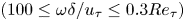$(100 \le \omega \delta /{u_\tau } \le 0.3R{e_\tau })$ originates from the overlap region $(50 \le {y^ + } \le 0.2R{e_\tau })$, where $R{e_\tau }\textrm{ }( = \delta {u_\tau }/\nu )$ is the friction Reynolds number and $\omega $ and $\delta $ are the frequency and boundary layer thickness, respectively. This is generally consistent with the proposition of Panton & Linebarger (1974). Later, Leclercq & Bohineust (2002) proposed via their model a logarithmic variation of scale-dependent convection velocity with frequency beyond $\omega \delta /{u_\tau } \approx 50$.

Recent experimental studies by Salze et al. (2014), Hu & Herr (2016), Joseph (2017) and Blitterswyk & Rocha (2017) are consistent with the abovementioned early findings regarding the scale-dependent convection velocity. Further, numerical studies also addressed the scale-dependent convection velocity for the wall pressure from either DNS (Choi & Moin 1990; Jeon et al. 1999; Bernardini & Pirozzoli 2011) or large eddy simulation (Viazzo, Dejoan & Schiestel 2001) with their results in general agreement with the experimental studies. However, such numerical studies have been performed at low Reynolds numbers. This limitation of the literature is among the motivations for the current study.

For the dependence of the convection velocity on the spanwise wavenumber, Kim & Hussain (1993) addressed it at a low Reynolds number from DNS. They showed that there is a strong dependence on the spanwise wavenumber but a rather weak dependence on the streamwise wavenumber. The dependence of the convection velocity on the spanwise wavenumber was also examined to some extent from the modelling study by Luhar et al. (2014). They obtained the pressure field in pipe flow in terms of the resolvent analysis at Reynolds numbers up to $R{e_\tau } = 5000$. A linear model was suggested based on the first singular response mode that was found to dominate the velocity field at a definite wavenumber–frequency combination. According to their model, they showed that modes with equal streamwise and azimuthal wavenumbers dominate the wall pressure field and propagate with velocities depending logarithmically on their size in agreement with Panton & Linebarger (1974). However, Luhar et al. (2014) did not present propagations of other different wall pressure scales.

1.1.2. Static pressure: Taylor's hypothesis and scale-dependent convection velocity

In wall-bounded flows, the static pressure is defined as the pressure across the boundary layer. There is an apparent lack of studies that verify the local mean velocity $U(y)$ for the convection velocity. One of the main reasons for this shortage is the difficulty inherent in measuring the pressure inside the flow field. Such measurements are difficult because the turbulent pressure fluctuations are subtle and can be distorted easily by ambient noise and probe intrusion (Tsuji et al. 2007; Naka et al. 2015). Tsuji et al. (2007) performed the first successful attempt to measure the static pressure within the turbulent boundary layer. The fundamental statistical quantities of the pressure, such as the mean, root mean square and power spectra, were investigated. Naka et al. (2015) used a similar probe to investigate spatio-temporal pressure–velocity correlations in the turbulent boundary layer. However, neither of the above two experimental studies discussed the application of $\textbf{TH}\textrm{-}{\boldsymbol{U}}$ to the static pressure.

From DNS in turbulent channel flow, Kim & Hussain (1993) addressed the application of Taylor's hypothesis of the pressure fluctuations at a low Reynolds number of $R{e_\tau } = 180$ where they computed the pressure convection velocity across the channel. They found that it is nearly equal to the local mean velocity $U(y)$ above ${y^ + } \approx 20$. Between the wall and ${y^ + } \approx 20$, the convection velocity has a constant value of approximately 0.75 times the centreline velocity. Since that time, no research has been done, from DNS, for the convection velocity of the static pressure in wall-bounded flows. Therefore, we were motivated to examine it for the static pressure.

Kim & Hussain (1993) and Luhar et al. (2014) examined the scale-dependent convection velocity of static pressure. From DNS, Kim & Hussain (1993) showed that it is only significant close to the wall with a stronger dependence on the spanwise wavenumber. They assigned that to the existence of structures with distinct spanwise scales within this region. Luhar et al. (2014), in their model, obtained the pressure field for motions with equal streamwise and azimuthal wavenumbers in pipe flow. They showed results for only two modes. Visual inspection of their figures 10(d) and 11(d) indicates that these two modes propagate with almost invariant velocities up to ${y^ + } \approx 10$ and 40, respectively, with larger velocity associated with the mode of the smaller wavenumber. Then, the convection velocities of the two modes coincide with the local mean velocity up to the pipe centre. However, Luhar et al. (2014) did not present the propagations of other different scales of static pressure.

1.2. Present contributions

In the first part of this study, we aim to answer the ongoing question about the value of Taylor convection velocity, as a function of wall distance, that can be applied for the hypothesis based on a comparison between the wavenumber and Taylor (frequency) premultiplied spectra. Both spectra are obtained from the same time series DNS datasets at Reynolds numbers up to $R{e_\tau } = 2000$, where $R{e_\tau } = h{u_\tau }/\nu $. Here, h is the channel half-depth and ${u_\tau }$ and $\nu $ represent the friction velocity and kinematic viscosity, respectively. The wall-normal locations and the wavenumber range where both spectra match each other are quantitively indicated. We examine both the local mean velocity $U(y)$ and the average convection velocity defined by Del Álamo & Jiménez (2009) ${C_p}(y)$ for the hypothesis, i.e. $\textbf{TH}\textrm{-}{\boldsymbol{U}}$ and $\textbf{TH}\textrm{-}{{C}_p}$. In the next part of this study, we discuss the difference between the wavenumber and frequency premultiplied spectra at any wall-normal location for any wavenumber range. The discussion is considered from the viewpoint of the turbulent structures associated with the pressure field. Then, a convection velocity that depends on both wall distance and scale is investigated and used in estimating the pressure spectra. Such velocity considers the convection velocities of the turbulent structures according to their contributions to the pressure variance.

Therefore, high-fidelity time series DNS datasets have been prepared to support such analysis of the pressure fluctuations in turbulent channel flow. The DNS datasets cover friction Reynolds numbers of $R{e_\tau } = 180$, $500$ and $2000$. This paper is organized as follows. Section 2 describes the DNS datasets utilized in the analysis. Section 3 describes the analytical methods for Taylor's hypothesis. The results of the convection velocity as a function of the distance from the wall are discussed in § 4. Section 5 addresses the classification and propagation of the pressure-relevant structures to obtain the scale-dependent convection velocity for the pressure field. Finally, we present our conclusions in § 6.

2. Turbulent channel flow database

The present analysis mainly needs spatio-temporal data from DNS of fully developed turbulent flow between two parallel planes. In this study, the three cases of $R180\textrm{ }(R{e_\tau } = 180)$, $R500\textrm{ }(R{e_\tau } = 500)$ and $R2000\textrm{ }(R{e_\tau } = 2000)$ in table 1 were newly carried out to obtain the spatio-temporal pressure field. In table 1, three Reynolds numbers of approximately $R{e_\tau } = 1000\textrm{ }(R1000)$ by Mehrez et al. (2019a), $4000\textrm{ }(R4000)$ by Mehrez, Yamamoto & Tsuji (2019b) and $8000\textrm{ }(R8000)$ by Kaneda & Yamamoto (2021) are also listed. In these three cases, high-resolution time series data were not obtained. Only their wavenumber spectra are used to discuss the spectral analysis of the pressure field in §§ 4 and 5.

Table 1. Summary of the DNS dataset parameters.

For all DNS databases, the coordinate system is $(x,y,z)$, where x, y and z represent the streamwise, wall-normal and spanwise coordinates, respectively. The computational domain sizes in the streamwise, wall-normal and spanwise directions are denoted as ${L_x}$, L_y and L_z, respectively. The flow was driven by a constant mean pressure gradient, and periodic boundary conditions were applied in the streamwise (x) and spanwise (z) directions, and no-slip/no-penetration boundary conditions were applied at the wall. The corresponding velocity fluctuations in the three directions are given by ${u_i}$, where $i = 1,2,3$ or $(u,v,w)$. The mean velocities in the three directions are expressed as ${U_i}$, where $i = 1,2,3$ or $(U,V,W)$. The instantaneous velocities are given by $u_i^t$, which has mean and fluctuating parts, and ${p^t}$ is the total pressure. For convenience, throughout the paper, a plus sign (+) indicates that the variable is scaled in wall units, where the friction velocity ${u_\tau }$ is the velocity scale and the viscous length $\nu /{u_\tau }$ represents the length scale. In addition, the wall pressure fluctuations are symbolized as ${p_w}$ to discriminate them from the static pressure fluctuations p (pressure across the channel).

As mentioned above, new DNSs were performed for the cases of R180, R500 and R2000 with large computational domains, ${L_x} \times {L_z} = (25.6 \times 9.6)h$ or $(8{\rm \pi} \times 3{\rm \pi})h$, and the four-dimensional spatio-temporal data of the pressure fields are obtained to analyse Taylor's hypothesis. The DNS uses a Fourier-spectral method in the wall-parallel, $x$ and z directions, and a second-order-accurate finite-difference method in the wall-normal, y direction. Alias errors associated with the pseudo-spectral method are removed using the $3/2$ rule. Poisson's equation for the pressure is solved using a tridiagonal matrix algorithm in Fourier space. The grid spacing is uniform in the streamwise and spanwise directions and is refined near the wall in the y direction to account for the large velocity gradient there. Hence, a hyperbolic tangent algebraic equation is applied for the grid spacing in the y direction. Table 1 shows the grid resolutions in the wall-parallel plane $\mathrm{(\Delta }{x^ + },\mathrm{\Delta }{z^ + })$, the grid resolution at the wall $\mathrm{\Delta }y_w^ + $ and the grid resolution at the centre of the channel $\mathrm{\Delta }y_c^ + $. Table 1 also provides the wave modes for the streamwise and spanwise directions $({N_x},{N_z})$ and the collocation points for the wall-normal direction ${N_y}$.

In the time integration for case R2000, the pressure and the other terms are time-advanced via the implicit Euler and second-order-accurate Adams–Bashforth methods, respectively. Alternatively, for cases R180 and R500, the viscous term is time-advanced via the Crank–Nicolson method, and the other terms are time-advanced as for case R2000. The simulation was run using a time step of $\mathrm{\Delta }{t^ + } = 0.18\;(\mathrm{\Delta }{t^ + } = \mathrm{\Delta }tu_\tau ^2/\nu )$ for cases R180 and R500 and $\mathrm{\Delta }{t^ + } = 0.0277$ for the higher Reynolds number of R2000. The total time integration lengths ${T^ + }$ normalized by the Reynolds number $({T^ + }/R{e_\tau } = T{u_\tau }/h)$ to obtain stable statistical results are summarized in table 1. The numerical accuracy of the present DNS database is confirmed via a comparison of statistical results with the previous DNS database under equivalent $R{e_\tau }$ conditions of $R{e_\tau } = 180$ and $2000$ (Kim, Moin & Moser 1987; Hoyas & Jiménez 2006; Bernardini, Pirozzoli & Orlandi 2014; Lee & Moser 2015; Yamamoto & Tsuji 2018).

The four-dimensional spatio-temporal data of the pressure field are stored with a regular time interval $\mathrm{\Delta }t_{st}^ + \textrm{ }(\mathrm{\Delta }t_{st}^ += \mathrm{\Delta }{t_{st}}u_\tau ^2/\nu )$. The values of $\mathrm{\Delta }t_{st}^ + $ are presented in table 1. The $\mathrm{\Delta }t_{st}^ + $ varies in each case but it is sufficiently smaller than the Kolmogorov time scale in wall units (${\equiv} {({\varepsilon ^ + })^{ - 1/2}} \ge 1.9$, where $\varepsilon $ is the energy dissipation rate per unit mass).

3. Analytical method for frozen turbulence hypothesis

3.1. Convection velocity

In this study, the average or overall convection velocity ${C_\phi }(y)$ is estimated as (Del Álamo & Jiménez 2009)

(3.1)\begin{equation}{C_\phi }(y) = - \frac{{\langle (\partial \phi /\partial t)(\partial \phi /\partial x)\rangle }}{{\langle {{(\partial \phi /\partial x)}^2}\rangle }}.\end{equation}

Here, the angle brackets $\langle \;\rangle $ denote ensemble averaging. Adopting the same definition as in Del Álamo & Jiménez (2009), we consider the $\omega $–${k_x}$ spectrum as

(3.2)\begin{equation}{\varPsi _{\phi \phi }}({k_x},y,{k_z},\omega ) = \langle \tilde{\phi }({k_x},y,{k_z},\omega ){\tilde{\phi }^\ast }({k_x},y,{k_z},\omega )\rangle .\end{equation}

Here, the asterisk denotes the conjugate and ${k_z}$ is the spanwise wavenumber. Note that we use a tilde to denote the Fourier transform with respect to the two homogeneous directions ($x$ and $z$) and time $(t)$. A carat $(\hat{} )$ is used for spatial Fourier coefficients that have only been transformed with respect to x and z but retain an explicit temporal dependence.

From the $\omega $–${k_x}$ spectrum, the scale-dependent convection velocity ${c_\phi }({k_x},y,{k_z})$ (time-averaged phase velocity of each spatial mode) is defined as

(3.3)\begin{equation}{c_\phi }({k_x},y,{k_z}) =- \frac{1}{{{k_x}}}{\; }\frac{{\int_{{\varOmega _\omega }} {\omega {\varPsi _{\phi \phi }}\textrm{(}{k_x},y,{k_z},\omega \textrm{)}\,\textrm{d}\omega } }}{{\int_{{\varOmega _\omega }} {{\varPsi _{\phi \phi }}\textrm{(}{k_x},y,{k_z},\omega \textrm{)}\,\textrm{d}\omega } }}.\end{equation}

Here, the frequency range ${\varOmega _\omega } \in [2{\rm \pi}/{T_N},{\rm \pi}/\Delta {t_{st}}]$ based on the wash-out time $({T_N} \approx {L_x}/{U_b})$ and the time interval $\mathrm{\Delta }{t_{st}}$ is adapted. In this study, the total time integration length ${T^ + }$ in table 1 is divided into overlapping time segments $T_N^ + $ (with $50\,\%$ overlap; see Choi & Moin 1990), and the spectra were averaged over all time segments.

The overall or average convection velocity ${C_\phi }(y)$ is also computed equivalently to (3.1) over ranges ${\varOmega _{{k_x}}}$ and ${\varOmega _{{k_z}}}$ of streamwise and spanwise wavenumbers, respectively, as (see Del Álamo & Jiménez (2009) for detailed derivation)

(3.4)\begin{equation}{C_\phi }(y) = \frac{{\int_{{\varOmega _{{k_z}}}} {\int_{{\varOmega _{{k_x}}}} {{c_\phi }({k_x},y,{k_z})} } |\hat{\phi }({k_x},y,{k_z}){\textrm{|}^2}k_x^2\,\textrm{d}{k_x}\,\textrm{d}{k_z}}}{{\int_{{\varOmega _{{k_z}}}} {\int_{{\varOmega _{{k_x}}}} {|\hat{\phi }({k_x},y,{k_z}){|^2}} } k_x^2\,\textrm{d}{k_x}\,\textrm{d}{k_z}}}.\end{equation}

3.2. Taylor spectra

Integrating equation (3.2) with respect to $\omega $ yields the two-dimensional (2-D) spectra in the wall-parallel plane $E_{\phi \phi }^{2D}({k_x},y,{k_z})$, which are discussed in § 5, as

(3.5)\begin{equation}E_{\phi \phi }^{2D}({k_x},y,{k_z}) = \int_{{\varOmega _\omega }} {{\varPsi _{\phi \phi }}\textrm{(}{k_x},y,{k_z},\omega \textrm{)}\,\textrm{d}\omega } .\end{equation}

In a like manner, the one-dimensional (1-D) wavenumber spectra in the streamwise direction ${E_{\phi \phi }}({k_x},y)$ (or streamwise spectra), and frequency spectra ${E_{\phi \phi }}(\omega ,y)$ are obtained as

(3.6)\begin{gather}{E_{\phi \phi }}({k_x},y) = \int_{{\varOmega _\omega }} {\int_{{\varOmega _{{k_z}}}} {{\varPsi _{\phi \phi }}({k_x},y,{k_z},\omega )\,\textrm{d}{k_z}\,\textrm{d}\omega } } ,\end{gather}

(3.7)\begin{gather}{E_{\phi \phi }}(\omega ,y) = \int_{{\varOmega _{{k_z}}}} {\int_{{\varOmega _{{k_x}}}} {{\varPsi _{\phi \phi }}({k_x},y,{k_z},\omega )\,\textrm{d}{k_x}\,\textrm{d}{k_z}} } .\end{gather}

In TH, the frequency spectra defined by (3.7) are converted to the streamwise wavenumber spectra via Taylor convection velocity ${U_T}$ as

(3.8)\begin{equation}E_{\phi \phi }^F(k_x^F,y) = {U_T}{E_{\phi \phi }}(\omega ,y).\end{equation}

Here, $E_{\phi \phi }^F(k_x^F,y)$ is called Taylor spectra (or frozen $\omega $-spectra), which are functions of the Taylor wavenumber $k_x^F = \omega /{U_T}$.

Similarly, the frozen ${k_x}$-spectra $E_{\phi \phi }^F({\omega ^F},y)$ are obtained from the streamwise spectra defined by (3.6) via ${U_T}$ as

(3.9)\begin{equation}E_{\phi \phi }^F({\omega ^F},y) = (1/{U_T}){E_{\phi \phi }}({k_x},y).\end{equation}

Here, ${\omega ^F} = {k_x}{U_T}$ is known as the Taylor frequency.

4. Results of Taylor's hypothesis for pressure fluctuations

4.1. Taylor's frozen hypothesis with local mean velocity $U(y)$ (TH-$\boldsymbol{U}$)

$\textbf{TH}\textrm{-}{\boldsymbol{U}}$ is verified here by comparing the streamwise spectra ${E_{pp}}({k_x},y)$ (equation (3.6)) to the frozen $\omega $-spectra $E_{pp}^F(k_x^F,y)$ (equation (3.8)) with the local mean velocity $U(y)$ applied for ${U_T}$. Even though the local mean velocity is quite small close to the wall, we apply it in computing the frozen $\omega $-spectra in (3.8). This serves to determine the wall-normal locations where the local mean velocity is not appropriate for ${U_T}$. The contour plots of the premultiplied 1-D streamwise spectra $k_x^ + E_{pp}^ += {k_x}{E_{pp}}/({\rho ^2}u_\tau ^4)$ and frozen $\omega $-spectra $k_x^{F + }E_{pp}^{F + } = k_x^FE_{pp}^F/({\rho ^2}u_\tau ^4)$ for the pressure fluctuations for R500 and R2000 are shown in figures 1(a-i) and 1(b-i), respectively. The spectra are plotted versus the streamwise wavelength and the distance from the wall.

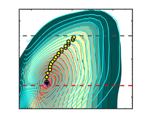
Figure 1. Results of $\textbf{TH}\textrm{-}{\boldsymbol{U}}$. (i) Contour lines of the premultiplied streamwise spectra ${k_x}{E_{pp}}/({\rho ^2}u_\tau ^4)$ (filled, black contour lines) and frozen $\omega $-spectra $k_x^F\; E_{pp}^F/({\rho ^2}u_\tau ^4)$ (open, cyan contour lines) of the pressure fluctuations versus ${y^ + }$ and the wavelength for (a) R500 and (b) R2000. In (a-i), the contour lines correspond to the values $[0.2\,:\,0.2\,:\,2.8]$, and they indicate the values 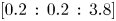$[0.2\,:\,0.2\,:\,3.8]$ in (b-i). In (i), the black and blue cross marks denote the peaks of the streamwise and frozen $\omega $-spectra, respectively. (ii) Contour lines of the difference ${D_{pp}}({k_x},y)$ between the streamwise spectra and frozen $\omega $-spectra for (a) R500 and (b) R2000. Black and blue colours correspond to positive and negative ${D_{pp}}({k_x},y)$, respectively. In (i) and (ii), the dashed red line indicates the wall-normal height ${y^ + } = 20$ and the grey line indicates the wall-normal distances ${y^ + } = 100$ in (a) and 400 in (b). In (a,b), the yellow circles indicate the ridges of the streamwise spectra with a streamwise wavelength of ${\lambda _{{x_r}}}(y)$.

In addition to the contour plots of the streamwise and frozen $\omega $-spectra, we present the contour maps for the difference between them in figure 1(ii) at the same Reynolds numbers. The difference (relative error) between the two spectra ${D_{pp}}({k_x},y)$ is defined as (Del Álamo & Jiménez 2009)

(4.1)\begin{equation}{D_{pp}}({k_x},y) = {k_x}\frac{{E_{pp}^F({k_x},y) - {E_{pp}}({k_x},y)}}{{\max [{k_x}{E_{pp}}({k_x},y)]}}.\end{equation}

It is noted that when computing ${D_{pp}}({k_x},y)$, a cubic spline interpolation scheme is applied for the frozen $\omega $-spectra to enable matching with the streamwise spectra.

Like the velocity fluctuations discussed in previous studies (e.g. Monty & Chong 2009; Wu et al. 2012; Squire et al. 2017), the contour lines of the streamwise and frozen $\omega $-spectra of the pressure field do not perfectly overlap each other for some regions normal to the wall. For the streamwise velocity fluctuations, Monty & Chong (2009) indicated differences between both spectra in the region below ${y^ + } = 50$ for streamwise wavelengths ${\lambda _x} > 4h$. But for the pressure field, the situation is different. From figures 1(a-i) and 1(b-i), we can discriminate three regions between the wall and channel centre based on the comparison between both spectra. The first region is the near-wall region below ${y^ + } \approx 20$. Within this region, the contour lines of the streamwise spectra are completely different from those of the frozen $\omega $-spectra. While the contour lines of the streamwise spectra tend to be vertical, indicating that the spectral energy of the pressure fluctuations resides in turbulent structures of nearly the same length scales (Jiménez & Hoyas 2008), the contour lines of the frozen $\omega $-spectra are inclined to the wall. This behaviour of the frozen $\omega $-spectra comes from the very small values of the local mean velocities in the near-wall region, which cannot reflect the convective nature of the pressure field. Hence, $\textbf{TH}\textrm{-}{\boldsymbol{U}}$ cannot be applied within this region as the difference between both spectra is quite large $(O({\pm} 50\,{\%}))$, as shown in figures 1(a-ii) and 1(b-ii).

The second region extends from ${y^ + } \approx 20$ to 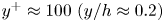${y^ + } \approx 100\textrm{ }(y/h \approx 0.2)$ for R500 in figure 1(a-i) and to 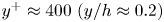${y^ + } \approx 400\textrm{ }(y/h \approx 0.2)$ for R2000 in figure 1(b-i). Generally, the streamwise and frozen $\omega $-spectra appear qualitatively similar. Within this range of Reynolds numbers, both spectra indicate the existence of only the inner peak reported in previous studies (Luhar et al. 2014; Tsuji, Marusic & Johansson 2016; Mehrez et al. 2019a). For both spectra, the streamwise wavelength associated with the inner peak is $\lambda _{{x_{peak}}}^ +\approx 250$. However, its location varies slightly among the spectra. For the streamwise spectra, it is located at approximately $y_{pea{k_T}}^ += 25$, while the frozen $\omega $-spectra suggest its location around $y_{pea{k_F}}^ += 21$. In addition, it is noted that the contour lines of the streamwise and frozen $\omega $-spectra match each other in the short-wavelength regime. In the long-wavelength regime, a slight difference between the two contour plots can be discerned. The short- and long-wavelength regimes are roughly discriminated in the figures based on the ridges of the streamwise spectra that indicate the peaks of the spectra at the various wall-normal locations (highlighted using yellow circles). The streamwise wavelength associated with the ridge of the streamwise spectra at each wall-normal location is denoted by ${\lambda _{{x_r}}}(y)$. It is worth mentioning that the relative error ${D_{pp}}({k_x},y)$ in this second region is of $O({\pm} 5\,{\%})$. However, it seems to increase with Reynolds number, as observed in figures 1(a-ii) and 1(b-ii).

The third region starts at ${y^ + } \approx 100\textrm{ }(y/h \approx 0.2)$ and 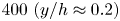$400\textrm{ }(y/h \approx 0.2)$ for R500 and R2000, respectively, and ends at the centre of the channel. The relative error between the two spectra almost vanishes, even for the higher Reynolds number R2000 (figure 1b-ii). The contour lines of the streamwise and frozen $\omega $-spectra overlap each other perfectly. Accordingly, $\textbf{TH}\textrm{-}{\boldsymbol{U}}$ is applicable in this region.

The behaviour indicated in the previous paragraphs may be perceived more clearly in figure 2, which shows the premultiplied streamwise spectra and frozen $\omega $-spectra versus the wavelength at three locations normal to the wall for R2000. The three locations shown in the figure represent the three regions described in the previous paragraphs. At $y/h \approx 0.2$, as shown in figure 2(c), a perfect consistency between the two spectra can be observed as they collapse quite well. However, this perfect overlap between the two spectra is only observed for short wavelengths at ${y^ + } \approx 70$ in figure 2(b). The spectra are different for long wavelengths. In addition, it is noted that the peak of the streamwise spectrum is attenuated relative to that of the frozen one.

Figure 2. Results of $\textbf{TH}\textrm{-}{\boldsymbol{U}}$. Profiles of the premultiplied streamwise spectra ${k_x}{E_{pp}}/({\rho ^2}u_\tau ^4)$ (solid curve) and frozen $\omega $-spectra $k_x^F\; E_{pp}^F/({\rho ^2}u_\tau ^4)$ (dotted curve) of the pressure fluctuations versus the wavelength for R2000 at (a–c) different wall-normal locations.

In figure 2(a), the frozen $\omega $-spectrum in the viscous sublayer at ${y^ + } \approx 5$ is shifted to shorter wavelengths than the streamwise spectrum. For the case of the velocity field, Squire et al. (2017) pointed out that this shift is attributed to a violation of $\textbf{TH}\textrm{-}{\boldsymbol{U}}$ where the velocity fluctuation intensity is high.

The results in figures 1 and 2 indicate that $\textbf{TH}\textrm{-}{\boldsymbol{U}}$ can be applied to the pressure field in channel flows above $y/h \approx 0.2$. Between ${y^ + } \approx 20$ and $y/h \approx 0.2$, $\textbf{TH}\textrm{-}{\boldsymbol{U}}$ is invalid for structures with wavelengths larger than approximately the ridges of the premultiplied spectra. Such structures seem to propagate with velocities that differ from the local mean. Generally, this deviation from $\textbf{TH}\textrm{-}{\boldsymbol{U}}$ does not exceed $5\,{\%}$ within this region, but it increases with Reynolds number. Finally, in the near-wall region up to ${y^ + } \approx 20$, $\textbf{TH}\textrm{-}{\boldsymbol{U}}$ is invalid where the maximum error of $O(50\,{\%})$. Therefore, the average pressure convection velocity ${C_p}(y)$ is estimated.

4.2. Taylor's frozen hypothesis with average (overall) convection velocity ${{C}_p}(y)$ (TH-${C_{\boldsymbol{p}}}$)

The results for the pressure average convection velocity ${C_p}(y)$ (computed using (3.4)) are shown in figure 3 for R180, R500 and R2000. In the figure, ${C_p}(y)$ is plotted versus the distance from the wall in inner and outer scaling in figures 3(a) and 3(b), respectively. Also shown in the figure is the local mean velocity at the same Reynolds numbers. The results of ${{C}_p}(y)$ are generally consistent with those of Kim & Hussain (1993) at $R{e_\tau } = 180$. From the wall up to ${y^ + } \approx 10$, the average convection velocity is larger than the mean velocity, being nearly constant with values of approximately $11.40{u_\tau }$–$12.05{u_\tau }$ $(0.55{U_{cl}}$–$0.66{U_{cl}})$. Geng et al. (2015) reported the Reynolds number dependence trend close to the wall upon estimating the convection velocities of the velocity fluctuations in channels. In their study, the convection velocities of the velocity components at $R{e_\tau } = 205$ overestimated those at $R{e_\tau } = 932$.

Figure 3. The average convection velocity of the pressure fluctuations ${C}_p^ + (y)$ for R180 (black), R500 (blue) and R2000 (brown) in (a) inner and (b) outer scaling for the wall distance. In the two panels, the local mean velocity ${U^ + }(y)$ is plotted versus the distance from the wall for R180 (triangles), R500 (squares) and R2000 (circles). (c) The difference between the average convection velocity of the pressure fluctuations and the local mean velocity ${C}_p^ + (y) - {U^ + }(y)$ for R180 (black), R500 (blue) and R2000 (brown) in outer scaling for the wall distance. The inset shows the difference ${C}_p^ + (y) - {U^ + }(y)$ in inner scaling for the wall distance. (d) The average convection velocities of the pressure fluctuations ${C}_p^ + (y)$ (brown), streamwise velocity ${C}_u^ + (y)$ (red), wall-normal velocity ${C}_v^ + (y)$ (magenta) and spanwise velocity ${C}_w^ + (y)$ (green), and the local mean velocity ${U^ + }(y)$ (open circles) for R2000 are plotted versus the distance from the wall in logarithmic scale. The average convection velocity of the streamwise velocity ${C}_u^ + (y)$ (filled circles) at $R{e_\tau } = 950$ from Del Álamo & Jiménez (2009) is plotted versus ${y^ + }$. The subscript $\phi $ in the $y$-axis label ${C}_\phi ^ + $ stands for p, u, v and w.

In addition, our result $(0.66{U_{cl}})$ for R180 is smaller than the value reported by Kim & Hussain (1993), which was $0.75{U_{cl}}$ at the same Reynolds number. This difference between the two values may be assigned to the difference between the method used here to compute the convection velocity and the method used in the aforementioned study. Del Álamo & Jiménez (2009) indicated that (3.4) weights ${{C}_p}(y)$ towards the convection velocities of high wavenumbers (containing higher spectral energy). However, Kim & Hussain (1993) computed the convection velocity from the space–time correlation using a time delay of $\mathrm{\Delta }{t^ + } = 18$, a value which they indicated to be too large for the high wavenumbers. Kim & Hussain (1993) examined the dependence of the convection velocity on the time delay $\mathrm{\Delta }{t^ + } = 3$, 18 and 27. The convection velocity in their study was found to change by about $18\,{\%}$ between $\mathrm{\Delta }{t^ + } = 3$ and 27 close to the wall (at ${y^ + } \approx 5$). Accordingly, it is inferred that ${{C}_p}(y)$ computed in this study is smaller than that provided by Kim & Hussain (1993) for locations close to the wall. For the same reasons, the reported average convection velocity of the wall pressure is smaller than that indicated by Choi & Moin (1990) and Jeon et al. (1999) ($0.72{U_{cl}}$ at $R{e_\tau } = 180$). From ${y^ + } \approx 10$ to ${y^ + } \approx 20$, the present convection velocity ${{C}_p}(y)$ increases very slightly until it becomes equal to ${U^ + }(y)$ at ${y^ + } \approx 20$, as shown in figure 3(a) for R180 and R2000. Beyond this location, the average convection velocity is consistent with the local mean velocity, being slightly smaller than ${U^ + }(y)$.

The difference between the pressure average convection velocity ${C}_p^ + (y)$ and the local men velocity ${U^ + }(y)$ is shown in figure 3(c) for R180, R500 and R2000. The difference is presented across the channel. It is clear in the figure that the difference is significant close to the wall which emphasizes that the local mean velocity is not applicable for representing Taylor convection velocity. Above the position ${y^ + } \approx 20$, the difference between ${C}_p^ + (y)$ and ${U^ + }(y)$ is small where it approaches a value of around $- 0.7$ in wall units for the different Reynolds numbers.

Superimposing the pressure average convection velocity on the local mean velocity helps to estimate the locations of the effective pressure field sources (Bull 1967; Blake 1970; Schewe 1983). For the wall pressure, Schewe (1983) indicated that the pressure convection velocity is equal to the local mean velocity at ${y^ + } = 21$, whereas Kim (1989) and Kim & Hussain (1993) estimated a higher location of ${y^ + } \approx 23$. Our results suggest the wall-normal location of ${y^ + } \approx 19.5$ for R180 and R2000 in close agreement with the aforementioned estimate by Schewe (1983). As pointed out by Kim (1989), it is inferred that the main contribution to the wall pressure comes from vortex-like structures, which are centred at ${y^ + } \approx 20$ in the near-wall region (Kim et al. 1987).

The average convection velocity of the pressure fluctuations ${C}_p^ + (y)$ is now compared with the convection velocities of the three velocity components at the same Reynolds number. The results are displayed in figure 3(d) for R2000. The average convection velocities of the pressure and velocity fields ${C}_\phi ^ + (y)$, where $\phi $ represents $p,u,v$ and w, are plotted versus the distance from the wall. The average convection velocities of the three velocity components are computed using the scheme presented by Del Álamo & Jiménez (2009), which we apply here to the pressure field (equation (3.4)). However, the scale-dependent convection velocities of the three velocity components are computed from the momentum equations derived by Del Álamo & Jiménez (2009) (their (2-11), (2-12), (2-13)) rather than the time series DNS dataset. Saving the time series data for the three velocity components in addition to the pressure field for our higher Reynolds number R2000 using the large computational domain $({L_x} \times {L_z} = (25.6 \times 9.6)h)$ requires a massive storage capacity (approximately 250 TB/turbulent field). Thus, for convenience, the time series dataset was saved only for the pressure field. For the velocity fluctuations, time realizations were saved at unequal time intervals.

The average convection velocity of the streamwise velocity in figure 3(d) matches that presented by Del Álamo & Jiménez (2009) at a lower Reynolds number of $R{e_\tau } = 950$ which is also included in figure 3(d) for comparison. In addition, the current investigation of the average convection velocities of the three velocity components agrees with the previous results presented by Kim & Hussain (1993) and Geng et al. (2015) at their lower Reynolds numbers of $R{e_\tau } = 180$ and up to 932, respectively. The average convection velocities of the three velocity components agree with each other remarkably well in the viscous sublayer below ${y^ + } \approx 5$. They are almost constant with a value of around $9{u_\tau }$. Beyond ${y^ + } \approx 5$, the convection velocities also increase slightly with the distance from the wall. Thus, the average convection velocity of the streamwise velocity seems to match the local mean velocity beyond ${y^ + } \approx 15$, whereas the other two velocity components have convection velocities that match the local mean velocity beyond ${y^ + } \approx 20$.

The larger values of the average convection velocities of the velocity fluctuations than the local mean velocity in the near-wall region originate from the footprint of large-scale structures, especially in the viscous sublayer. For u fluctuations, eddies with ${\lambda _x} \ge 2h$ and ${\lambda _z} \ge 0.4h$ contribute to the convection velocity in the near-wall region and propagate with a uniform velocity scaled with the bulk velocity (Del Álamo & Jiménez 2009). From the recent input–output approach developed by Liu & Gayme (2020) to estimate the convection velocity based on the linearized Navier–Stokes equations, a range of large-scale structures was quantified with dimensions ${y^ + }\sim \lambda _z^ +{\sim} {(\lambda _x^ + )^{2/3}}$. They inferred that these structures are self-similar in the cross-plane and retain a wall-normal coherence with an inclination to the wall consistent with the attached eddy hypothesis of Townsend (1976).

Remarkably, the average convection velocity of the pressure field ${C}_p^ + (y)$ is larger than the convection velocities of the three velocity components close to the wall (figure 3d). This larger value of the pressure convection velocity is consistent with the global features of the pressure fluctuations, as indicated by Poisson's equation for the pressure (Willmarth 1975; Kim 1989). Sillero, Jiménez & Moser (2014) showed that pressure correlation retains a stronger correlation in the wall-normal direction than velocity correlations. From Poisson's pressure equation analysis by Green's function, Jiménez & Hoyas (2008) identified two mean structures concerned with the pressure fluctuations. The first one is an energetic localized structure in the near-wall and logarithmic regions, while the second one is a large-scale structure $O(h)$ that extends across the entire flow thickness. Sillero et al. (2014) quantified the first and second structures in terms of strong and weak correlations, respectively. Therefore, the convection velocity of the pressure field is elevated in the near-wall region with multiple scale contributions. Pressure-relevant structures are discussed in § 5.

We investigated the average pressure convection velocity ${{C}_p}(y)$ across the entire flow. The frozen $\omega $-spectra $E_{pp}^F(k_x^F,y)$ in (3.8) are computed from ${{C}_p}(y)$ which is applied for ${U_T}$. The results of $\textbf{TH}\textrm{-}{{C}_p}$ are shown in figure 4. In comparison with figure 1, the collapse between both spectra in the near wall-region below ${y^ + } = 20$ is improved significantly and the difference between them decreased to a value of $O(10\,\%)$ for its maximum. This improvement is expected from figure 3(c) for the difference between ${{C}_p}(y)$ and $U(y)$. As indicated in figures 4(a-ii) and 4(b-ii), the difference exists around the ridges of the streamwise spectra and for larger scales. On the other hand, the small difference between the two velocities for the region above ${y^ + } = 20$ does not have an impact on the computed frozen $\omega $-spectra as their values are the same as in figure 1. Therefore, above ${y^ + } = 20$, $\textbf{TH}\textrm{-}{{C}_p}$ yields the same results as $\textbf{TH}\textrm{-}{\boldsymbol{U}}$, as shown in figure 4.

Figure 4. Results of $\textbf{TH}\textrm{-}{{C}_p}$. Same as figure 1. However, the contour lines of the frozen spectra are indicated by red colour.

Based on the above observations, the average convection velocity ${{C}_p}(y)$ is better for representing the Taylor convection velocity for the pressure fluctuations compared with the local mean velocity. However, it is difficult to compute it from numerical simulations especially when Reynolds number increases. Besides, it cannot be obtained from experiments for static pressure. Therefore, we define a simply modelled convection velocity for the pressure field ${C}_p^M(y)$ derived from both the local mean velocity $U(y)$ and average convection velocity ${{C}_p}(y)$. It is discussed in the next subsection.

4.3. Taylor's frozen hypothesis with modelled convection velocity ${C}_p^M(y)$ (TH-${C}_{\boldsymbol{p}}^{\boldsymbol{M}}$)

The modelled convection velocity is defined as

(4.2)\begin{equation}{C}_p^M(y) = \left\{ {\begin{array}{*{20}{@{}ll}} {U({y^ + } = 20)}&{0 \le {y^ + } < 20,}\\ {U(y)}&{20 \le {y^ + } \le {h^ + }.} \end{array}} \right.\end{equation}

In this model, above ${y^ + } = 20$, the local mean velocity is adopted for the convection velocity. Below this position, the convection can be regarded as constant with a value that equals the local mean velocity at ${y^ + } = 20$. For this velocity, Taylor's hypothesis is defined as $\textbf{TH}\textrm{-}{{C}}_{\boldsymbol{p}}^{\boldsymbol{M}}$ and is considered in both wavenumber and frequency spaces.

4.3.1. Wavenumber space

The frozen $\omega $-spectra $E_{pp}^F(k_x^F,y)$ in (3.8) are computed from ${C}_p^M(y)$ which is applied for ${U_T}$. According to (4.2), we present the results for the region below ${y^ + } = 20$. Specifically, figures 5(a) and 5(b) show the comparison between the streamwise spectra ${k_x}{E_{pp}}/({\rho ^2}u_\tau ^4)$ and the frozen ones $k_x^FE_{pp}^F/({\rho ^2}u_\tau ^4)$ for R500 and R2000, respectively. The same results are obtained as in figure 4 where around the ridges of the streamwise spectra and for larger scales, the difference between both spectra still exists.

Figure 5. Results of $\textbf{TH}\textrm{-}{{C}}_p^M$. Same as figure 1. However, the results are shown for the region $0 \le {y^ + } \le 20$.

This is further clarified in figure 6(a), where the wall pressure premultiplied streamwise and frozen spectra are displayed (streamwise spectrum: $k_x^ + {\; }E_{{p_w}{p_w}}^ += {k_x}{\; }{E_{pp}}({k_x},y = 0)/({\rho ^2}u_\tau ^4)$; frozen spectrum: $k_x^{F + }\; E_{{p_w}{p_w}}^{F + } = k_x^FE_{pp}^F(k_x^F,y = 0)/({\rho ^2}u_\tau ^4)$). The two dashed lines shown in the figure are associated with the two length scales $\lambda _{{x_{in}}}^ += 250$ and ${\lambda _{{x_{out}}}}/h = 1$ (for R2000). We define these length scales upon our analysis of the wall pressure structures classification in § 5. Several notes can be derived from the figure. First, both spectra, streamwise and frozen, peak at the same length scale of $\lambda _{{x_r}}^ + \textrm{(}y = 0\textrm{)} \approx 250$, which equals the length scale of the inner peak of the premultiplied spectra shown in figure 1(i) that occurs at $y_{pea{k_T}}^ +\approx 25$. This indicates that specific structures dominate the pressure field from the wall to ${y^ + } \approx 25$. Second, the frozen spectrum's peak exaggerates the streamwise one's peak, although both spectra peak at the same length scale. Third, an opposed behaviour for the large-scale structures is observed where an underestimation of the frozen spectrum with respect to the streamwise one can be discerned. These differences between the spectra arise from the various structures that contribute to the wall pressure fluctuations and propagate with different convection velocities as clarified in § 5. This yields a relative error ${D_{{p_w}{p_w}}}({k_x}) = {D_{pp}}({k_x},y = 0)$ between the spectra of $O(10\,{\%})$ for its maximum value as shown in figure 6(b).

Figure 6. Results of $\textbf{TH}\textrm{-}{{C}}_p^M$. (a) The profiles of the premultiplied streamwise ${k_x}{E_{{p_w}{p_w}}}/({\rho ^2}u_\tau ^4) = {k_x}\; {E_{pp}}({k_x},y = 0)/({\rho ^2}u_\tau ^4)$ (solid curve) and frozen $k_x^F\; E_{{p_w}{p_w}}^F/({\rho ^2}u_\tau ^4) = k_x^F\; E_{pp}^F(k_x^F,y = 0)/({\rho ^2}u_\tau ^4)$ (dotted curve) spectra of the wall pressure fluctuations versus the streamwise wavelength in inner scaling $\lambda _x^ + $ for R500 (blue) and R2000 (brown). The top horizontal axis is the streamwise wavelength in outer scaling ${\lambda _x}/h$ for R2000. The two dashed vertical lines correspond to $\lambda _{{x_{in}}}^ += 250$ and ${\lambda _{{x_{out}}}}/h = 1$ ($\lambda _{{x_{out}}}^ += 2000$ for R2000). (b) The difference between the streamwise and frozen $\omega $-spectra of the wall pressure ${D_{{p_w}{p_w}}}({k_x}) = {D_{pp}}({k_x},y = 0)$ at R500 (blue) and R2000 (brown). The yellow circle in (a) indicates the ridge of the streamwise spectrum for R2000.

4.3.2. Frequency domain

To test the application of $\textbf{TH}\textrm{-}{{C}}_p^M$ further, a comparison with the experimental wall pressure results of Tsuji et al. (2007) is performed. For this, we move to the frequency domain. Figure 7 presents the frequency spectrum of the wall pressure ${E_{{p_w}{p_w}}}(\omega ) = {E_{pp}}(\omega ,y = 0)$ (equation (3.7)) for R500 and R2000. In addition, figure 7 presents the results of the frozen ${k_x}$-spectrum (equation (3.9) with ${C}_p^M(y)$ applied for ${U_T}$) for the wall pressure $E_{{p_w}{p_w}}^F({\omega ^F}) = E_{pp}^F({\omega ^F},y = 0)$ for cases R500, R2000, R4000 and R8000. The frequency spectrum of the wall pressure for a turbulent boundary layer at $R{e_\tau } = 1760$, 2100 and 3883 from Tsuji et al. (2007) is also shown in the figure. All spectra are normalized with the inner variables ${u_\tau }$ and $\nu $, and are presented as functions of $\omega \nu /u_\tau ^2$. Thus, the collapse of the spectra is observed in the high-frequency range for all Reynolds numbers. This indicates that near-wall-region structures dominate the wall pressure fluctuations within this frequency range (Farabee & Casarella 1991; Tsuji et al. 2007).

Figure 7. Results of $\textbf{TH}\textrm{-}{{C}}_p^M$. Wall pressure frequency spectra ${E_{{p_w}{p_w}}}(\omega )/({\rho ^2}u_\tau ^2\nu ) = {E_{pp}}(\omega ,y = 0)/({\rho ^2}u_\tau ^2\nu )$ (dashed) and frozen ${k_x}$-spectra $E_{{p_w}{p_w}}^F\; ({\omega ^F})/({\rho ^2}u_\tau ^2\nu ) = E_{pp}^F\; ({\omega ^F},y = 0)/({\rho ^2}u_\tau ^2\nu )$ (solid) versus $\omega \nu /u_\tau ^2$ for R500 (blue), R2000 (brown), R4000 (green) and R8000 (magenta). Wall pressure spectra at $R{e_\tau } = 1760$, 2100 and 3883 from Tsuji et al. (2007) are shown in grey. The two solid, vertical grey lines correspond to $\omega \nu /u_\tau ^2 = 0.013$ and 0.189, while the two dashed ones correspond to $\omega \nu /u_\tau ^2 = {\omega _{in}}\nu /u_\tau ^2$ and ${\omega _{out}}\nu /u_\tau ^2$ with ${\omega _{in}} = (2{\rm \pi}/{\lambda _{{x_{in}}}}){C}_{{p_w}}^M$ and ${\omega _{out}} = (2{\rm \pi}/{\lambda _{{x_{out}}}}){C}_{{p_w}}^M$, where 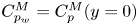${C}_{{p_w}}^M = {C}_p^M(y = 0)$, $\lambda _{{x_{in}}}^ += 250$ and ${\lambda _{{x_{out}}}}/h = 1$ ($\lambda _{{x_{out}}}^ += 2000$ for R2000).

Instead of observing the power-law spectrum ${\omega ^{ - 1.0}}$ predicted by Bradshaw (1967), Tsuji et al. (2007) inferred the existence of a power-law spectrum corresponding to ${\omega ^{ - 0.7}}$ within the frequency range of $0.013 \le \omega \nu /u_\tau ^2 \le 0.189$. This frequency range is presented in figure 7. Tsuji et al. (2007) concluded that the wall pressure spectra with an exponent of $( - 1.0)$ occur only at high Reynolds numbers $(R{e_\tau } \approx O({10^6}))$, which were examined later by Klewicki, Priyadarshana & Metzger (2008). Our DNS results in figure 7 indicate that both frequency and frozen ${k_x}$-spectra exhibit ${\omega ^{ - 0.7}}$ spectra over the frequency range ${\omega _{out}}\nu /u_\tau ^2 \le \omega \nu /u_\tau ^2 \le {\omega _{in}}\nu /u_\tau ^2$ for R2000. The bounds ${\omega _{in}}$ and ${\omega _{out}}$ correspond to the two length scales ${\lambda _{{x_{in}}}}$ and ${\lambda _{{x_{out}}}}$ in figure 6 such that ${\omega _{in}} = (2{\rm \pi}/{\lambda _{{x_{in}}}}){C}_{{p_w}}^M$ and ${\omega _{out}} = (2{\rm \pi}/{\lambda _{{x_{out}}}}){C}_{{p_w}}^M$, where ${C}_{{p_w}}^M = {C}_p^M(y = 0)$. It is noted that R500 exhibits ${\omega ^{ - 0.7}}$ spectra over a very narrow range. The reasoning behind this narrow range is clarified later in the discussion about classifying the wall pressure structures in § 5.

Using the modelled convection velocity for the wall pressure allows ${\omega ^{ - 0.7}}$ spectra to be identified within our DNS for R4000, consistent with the experimental results at the nearly same Reynolds number. As expected, the spectral region corresponding to ${\omega ^{ - 0.7}}$ spectra bounded by ${\omega _{in}}$ and ${\omega _{out}}$ increases with Reynolds number. On the other hand, for the higher Reynolds number, R8000, the slope increases slightly towards $( - 1.0)$, although we do not reach the theoretical slope discussed by Bradshaw (1967). Panton, Lee & Moser (2017) also observed an increase in the slope of the wall pressure spectrum for their high Reynolds number of $R{e_\tau } = 5200$.

In the low-frequency range, there is a difference between the experimental boundary layer results and the channel results from DNS at the same Reynolds number. In figure 7, the results of channel flow of R2000 (dashed brown line from present DNS) and the results of boundary layer at $R{e_\tau } = 2100$ from Tsuji et al. (2007) are almost at the same Reynolds number. Despite that, there is no collapse between both spectra in the low-frequency range. The low-frequency range of the spectra is associated with structures from the outer layer (Farabee & Casarella 1991). As a result, this difference is expected since the outer layer large-scale structures in boundary layers (with outside potential field) are different from those in turbulent channels (Sillero et al. 2014), and they affect the pressure statistics (Panton et al. 2017). Besides, for the channel DNS results, there is an obvious difference in the low-frequency range between frequency and frozen ${k_x}$-spectra for either R500 (solid and dashed blue lines) or R2000 (solid and dashed brown lines). Since both spectra (frequency and frozen ${k_x}$-spectra) are at the same Reynolds number (either $R{e_\tau } = 500$ or 2000) for the same flow field (channel) from the same dataset (DNS), the only reasoning we have here is applying Taylor's hypothesis with the convection velocity ${C}_{{p_w}}^M$.

In summary, $\textbf{TH}\textrm{-}{{C}}_p^M$ is better than $\textbf{TH}\textrm{-}{\boldsymbol{U}}$ in the near-wall region below ${y^ + } = 20$. However, $\textbf{TH}\textrm{-}{{C}}_p^M$ produces an error of $O(10\,{\%})$ for its maximum value, and it increases with Reynolds number. Also, $\textbf{TH}\textrm{-}{{C}}_p^M$ produces an error of $O (5\,{\%})$ for its maximum in the region between ${y^ + } = 20$ and $y/h = 0.2$ for structures with wavelengths associated with the ridges of the premultiplied streamwise spectra and larger ones (same as $\textbf{TH}\textrm{-}{\boldsymbol{U}}$ according to (4.2)). Therefore, in the next section, we examine the scale-dependent convection velocity for the conversion between time and space domains.

5. Scale-dependent convection velocity for pressure fluctuations (from the wall to $y/h = 0.2$)

It was found from the previous section that a difference between the streamwise and frozen spectra occurs for some wavelengths. For the streamwise velocity fluctuations, Del Álamo & Jiménez (2009) indicated that the difference between both spectra is associated with large-scale structures of wavelengths $({\lambda _x},{\lambda _z}) \ge (2h,0.4h)$. They indicated that such structures propagate with velocities scaled with the bulk velocity ${U_b}$. The question is: ‘does the difference between both spectra for the pressure field occur for the same “large-scale” structures?’. From three-dimensional two-point correlation analysis in physical space, Sillero et al. (2014) indicated that the pressure correlations differ from those of streamwise velocity fluctuations and resemble those of spanwise and wall-normal velocity components. Additionally, from proper orthogonal decomposition, Jiménez (2018) indicated that the pressure is dominated by structures different from those of u fluctuations. Hence, the large-scale structures defined by Del Álamo & Jiménez (2009) for u fluctuations cannot be employed for the pressure, and we should provide a clear definition for large-scale structures of the pressure fluctuations.

The classifications of the pressure structures can be performed by addressing the scaling of the 2-D pressure spectra. After that, we address the propagation of each class of pressure structures. Then, the appropriate scale-dependent convection velocity for the pressure field is proposed by considering the velocities of the different classes of structures.

5.1. Pressure structure classification

Here, we discuss the 2-D spectrum of the wall pressure in the wall-parallel plane $E_{{p_w}{p_w}}^{2D}({k_x},{k_z}) = E_{pp}^{2D}({k_x},y = 0,{k_z})$. The premultiplied 2-D spectrum of the wall pressure ${k_x}{k_z}E_{{p_w}{p_w}}^{2D}/({\rho ^2}u_\tau ^4)$ is plotted versus the streamwise and spanwise wavelengths in inner and outer scaling in figures 8(a) and 8(b), respectively. Following Jiménez & Hoyas (2008), the contour lines of R500 and R2000 are shown, where the contour lines are normalized with their maxima for each Reynolds number. As seen in the figure and as documented previously (Jiménez & Hoyas 2008; Luhar et al. 2014), the 2-D pressure spectra are mostly aligned along the equilateral line ${\lambda _z} = {\lambda _x}$. Further, the spectral energy of the wall pressure is relevant to length scales different from those of u fluctuations at ${y^ + } = 15$ (close to the wall).

Figure 8. Contour lines of the premultiplied 2-D spectra of the wall pressure ${k_x}{k_z}E_{{p_w}{p_w}}^{2D}/({\rho ^2}u_\tau ^4) = {k_x}{k_z}E_{pp}^{2D}({k_x},y = 0,{k_z})/({\rho ^2}u_\tau ^4)$ versus the streamwise and spanwise wavelengths in (a) inner and (b) outer scaling for R500 (blue) and R2000 (brown). The diagonal dashed-dotted line is related to ${\lambda _z} = {\lambda _x}$. The top and right axes in (a) are the wavelengths in outer scaling corresponding to R2000. Contour lines in (a) and (b) correspond to the values $\{ 0.05,{\; }0.1,{\; }0.3,{\; }0.5,{\; }0.7\} $ and $\{ 0.02,{\; }0.04,{\; }0.06,{\; }0.1,0.15,{\; }0.6\} $, respectively, times the maximum of the contours at each Reynolds number. In (a), the two dashed vertical lines correspond to $\lambda _{{x_{in}}}^ += 250$ and ${\lambda _{{x_{out}}}}/h = 1$ ($\lambda _{{x_{out}}}^ += 2000$ for R2000) and the two horizontal ones correspond to $\lambda _{{z_{in}}}^ += 250$ and ${\lambda _{{z_{out}}}}/h = 1$ ($\lambda _{{z_{out}}}^ += 2000$ for R2000). The yellow circle in (a) represents the ridge of the premultiplied 1-D streamwise wall pressure spectrum ${k_x}{E_{{p_w}{p_w}}}/({\rho ^2}u_\tau ^4)$. In (b), the dashed vertical and horizontal lines are related to ${\lambda _{{x_{out}}}}/h = 1$ and ${\lambda _{{z_{out}}}}/h = 1$, respectively. The symbols: ‘S’, ‘I’ and ‘L’ denote the small-, intermediate- and large-scale regions, respectively.

In figures 8(a) and 8(b), R500 and R2000 contour lines that collapse with each other are highlighted using thick colours. In figure 8(a), the collapse of the contour lines of the spectra for R500 and R2000 is noted for small-scale structures bounded by $\lambda _x^ + \le \lambda _{{x_{in}}}^ + $ and $\lambda _z^ + \le \lambda _{{z_{in}}}^ + $ upon normalizing the wavelengths with the inner variables, where 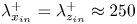$\lambda _{{x_{in}}}^ += \lambda _{{z_{in}}}^ +\approx 250$. Thus, we define the ‘inner’ streamwise and spanwise separation length scales as $\lambda _{{x_{in}}}^ += 250$ and $\lambda _{{z_{in}}}^ += 250$, respectively. The inner separation length scales are selected at this value, which indicates the streamwise wavelength $\lambda _{{x_r}}^ + (y = 0) = 250$ associated with the ridge of the premultiplied 1-D spectrum (figure 6a). With the alignment of the premultiplied 2-D spectrum along ${\lambda _z} = {\lambda _x}$, it is indicated that 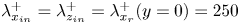$\lambda _{{x_{in}}}^ += \lambda _{{z_{in}}}^ += \lambda _{{x_r}}^ + (y = 0) = 250$. Selecting the inner separation length scales $(\lambda _{{x_{in}}}^ + ,\lambda _{{z_{in}}}^ + )$ with this value guarantees including all length scales with their spectra collapsing with each other for the two Reynolds numbers. In figure 8(a), the collapse of the spectra is observed at different length scales for the different values of the contour lines. When the spectral density decreases (low value of the contour lines), the streamwise and spanwise wavelengths at which the contours overlap each other increase. The ‘inner’ separation length scales $(\lambda _{{x_{in}}}^ + ,\lambda _{{z_{in}}}^ + )$, chosen at this value of $\lambda _{{x_r}}^ + (y = 0) = 250$, match the collapse of both strong spectral densities (high values of the contour lines) and weak ones (low values of the contour lines).

In figure 8(b), with the outer scaling of the coordinates, a collapse between the spectra is noted for large-scale structures. Such outer scaling of the spectra is achieved for streamwise and spanwise length scales larger than approximately h. Accordingly, the ‘outer’ streamwise and spanwise separation length scales are defined as ${\lambda _{{x_{out}}}} = {\lambda _{{z_{out}}}} = h$. It is noted that the collapse of the spectra for large-scale structures occurs for small spectral densities (low values of the contour lines). Figure 8(b) shows that contour lines associated with $0.6$ do not overlap for the two Reynolds numbers. That is why different contour levels are shown in figure 8(b) compared with figure 8(a).

Based on the abovementioned observations, we can classify the structures associated with the wall pressure into three categories based on their wall-parallel length scales: (1) small-scale structures with ${\lambda _x} \le {\lambda _{{x_{in}}}}$ and ${\lambda _z} \le {\lambda _{{z_{in}}}}$, (2) large-scale structures with ${\lambda _x} \ge {\lambda _{{x_{out}}}}$ and ${\lambda _z} \ge {\lambda _{{z_{out}}}}$ and (3) intermediate-scale structures at other length scales. Such classifications are like that proposed by Farabee & Casarella (1991) in the frequency domain. However, we classify the structures based on their sizes in the wall-parallel plane, as shown in figure 8(a). Additionally, the large-scale structures defined here agree with the quantification of the pressure structures indicated previously by Jiménez & Hoyas (2008) and confirmed by Sillero et al. (2014). However, both previous studies did not discriminate between small- and intermediate-scale structures as they considered them one class. Besides, the previous study by Mehrez et al. (2019a) indicated such separation scales for large-scale structures based on the analysis of the higher-order moments of the pressure field in turbulent channel flow.

It is worth mentioning that the intermediate-scale structures for streamwise wavelengths between ${\lambda _{{x_{in}}}}$ and ${\lambda _{{x_{out}}}}$ are associated with the ${\omega ^{ - 0.7}}$ spectra of the frequency spectra shown in figure 7. When Reynolds number decreases, this range of length scales decreases as well. That is why R500 exhibits ${\omega ^{ - 0.7}}$ spectra over a narrow range in figure 7.

We now extend the concept of structure classification from the 2-D spectra to the static pressure fluctuations. In the first step, we determine the separation length scales $({\lambda _{{x_{in}}}},\; {\lambda _{{z_{in}}}})$ and $({\lambda _{{x_{out}}}},\; {\lambda _{{z_{out}}}})$. The ridge of the premultiplied 1-D spectra of the pressure $k_x^ + E_{pp}^ + ({k_x},y)$ is examined for $({\lambda _{{x_{in}}}},\; {\lambda _{{z_{in}}}})$, and h is examined for $({\lambda _{{x_{out}}}},\; {\lambda _{{z_{out}}}})$. Hence, we can identify the three types of structures.

Figure 9 is the same as figure 8, except that the results are shown for the pressure field at ${y^ + } = 100$. In figure 9(a), the inner separation length scales are determined as $\lambda _{{x_{in}}}^ + ({y^ + } = 100) = \lambda _{{z_{in}}}^ + ({y^ + } = 100) = \lambda _{{x_r}}^ + ({y^ + } = 100)$ where the collapse of the spectra is discerned. In this regard, ${\lambda _{{x_{in}}}}$ and ${\lambda _{{z_{in}}}}$ increase with the distance from the wall y. Accordingly, the range of length scales of the small-scale structures increases with the distance from the wall y. However, the outer separation length scales $({\lambda _{{x_{out}}}},\; {\lambda _{{z_{out}}}})$ are almost invariant when normalized by h with the collapse of the spectra in figure 9(b). This means that the large-scale structures reside over the same range of length scales as for the wall pressure.

Figure 9. As figure 8 except that the results are shown at ${y^ + } = 100$. The yellow circle in (a) represents the ridge of the premultiplied 1-D streamwise pressure spectrum ${k_x}{E_{pp}}/({\rho ^2}u_\tau ^4)$ at ${y^ + } = 100$.

The classification of structures adopted here is not interpreted in any physical space. However, the pressure structure classification in Fourier space presented here seems relevant to the physical structures addressed in previous studies (Kobashi & Ichijo 1990; Ahn et al. 2010; Ghaemi & Scarano 2013; Mehrez et al. 2019a,b). The connection between pressure structure classification employed in the present study and pressure structures in physical space is of significance and will be considered in the future.

Once we have classified the pressure structures, it is significant to address their contributions to the spectral energy of the pressure field. We discuss that in the next subsection.

5.2. Structures’ contributions to the pressure variance

We identify the contribution of each class of structures to the pressure variance $\langle \,{p^{{ + ^2}}}\rangle $ between the wall and $y/h = 0.2$. The contribution from each class to the spectral energy of the wall pressure (wall pressure variance $\langle \,p_w^{{ + ^2}}\rangle = \langle \,p_w^2\rangle /({\rho ^2}u_\tau ^4)$) is shown in figure 10(a) for various Reynolds numbers. This is determined by computing the variance of the wall pressure associated with each category. The wall pressure variances associated with small-, intermediate- and large-scale structures are denoted by $\langle \,p_w^{{ + ^2}}\rangle {|_S}$, $\langle \,p_w^{{ + ^2}}\rangle {|_I}$ and $\langle \,p_w^{{ + ^2}}\rangle {|_L}$, respectively. The figure also shows the total wall pressure variance $\langle \,p_w^{{ + ^2}}\rangle $. The wall pressure variance results of Lee & Moser (2015) are also included. As shown in figure 10(a), the intermediate-scale structures seem to maintain a higher contribution to the wall pressure variance than the small- and large-scale structures for the different Reynolds numbers. For instance, the relative contributions to the total wall pressure variance from the small-scale $(\langle \,p_w^{{ + ^2}}\rangle {|_S}/\langle \,p_w^{{ + ^2}}\rangle )$, intermediate-scale $(\langle \,p_w^{{ + ^2}}\rangle {|_I}/\langle \,p_w^{{ + ^2}}\rangle )$ and large-scale $(\langle \,p_w^{{ + ^2}}\rangle {|_L}/\langle \,p_w^{{ + ^2}}\rangle )$ structures for R2000 are approximately 16 %, 73 % and 11 %, respectively. It is noted that when Reynolds number increases, the contribution from the intermediate-scale class increases, while the contributions from the other two classes are nearly invariant.

Figure 10. (a) Wall pressure variance $\langle \,p_w^{{ + ^2}}\rangle $ versus Reynolds number from the present DNS (yellow squares) and from Lee & Moser (2015) (red stars). Wall pressure variance associated with small-scale $\langle \,p_w^{{ + ^2}}\rangle {|_S}$ (green circles), intermediate-scale $\langle \,p_w^{{ + ^2}}\rangle {|_I}$ (blue triangles) and large-scale $\langle \,p_w^{{ + ^2}}\rangle {|_L}$ (red diamonds) structures. Solid red and green lines are the relations presented by Farabee & Casarella (1991), 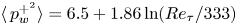$\langle \,p_w^{{ + ^2}}\rangle = 6.5 + 1.86\ln (R{e_\tau }/333)$, and Sillero et al. (2013), $\langle \,p_w^{{ + ^2}}\rangle =- 9.5 + 2.31\ln (R{e_\tau })$, respectively. The dashed cyan line is the fit of $\langle \,p_w^{{ + ^2}}\rangle {|_I}$ with Reynolds number, $\langle \,p_w^{{ + ^2}}\rangle {|_I} =- 9.5 + 2.03\ln (R{e_\tau })$. (b) Pressure variance $\langle \,{p^{{ + ^2}}}\rangle $ versus the distance from the wall for R500 (blue), R1000 (red), R2000 (brown) and R4000 (green). The panel displays the total pressure $\langle \,{p^{{ + ^2}}}\rangle $ (solid), small-scale $\langle \,{p^{{ + ^2}}}\rangle {|_S}$ (dotted), intermediate-scale $\langle \,{p^{{ + ^2}}}\rangle {|_I}$ (dashed) and large-scale $\langle \,{p^{{ + ^2}}}\rangle {|_L}$ (dashed-dotted) pressure variances. The dashed cyan line is the logarithmic slope ${A_p} = 2.511$.

With their large contribution to the wall pressure variance, the intermediate-scale structures are mainly responsible for the logarithmic dependence of the total wall pressure variance with Reynolds number. The Reynolds number dependence of the total wall pressure variance $\langle \,p_w^{{ + ^2}}\rangle $ is indicated in figure 10(a) where it maintains a logarithmic relation with Reynolds number (Willmarth 1975). Farabee & Casarella (1991) derived the following relation between $\langle \,p_w^{{ + ^2}}\rangle $ and Reynolds number: $\langle \,p_w^{{ + ^2}}\rangle = 6.5 + 1.86\ln (R{e_\tau }/333)$ for $R{e_\tau } > 333$, based on integrating the frequency spectra from 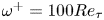${\omega ^ + } = 100R{e_\tau }$ to 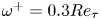${\omega ^ + } = 0.3R{e_\tau }$. They assumed ${\omega ^{ - 1}}$ spectra within this frequency range. The relation presented by Farabee & Casarella (1991), $\langle \,p_w^{{ + ^2}}\rangle = 6.5 + 1.86\ln (R{e_\tau }/333)$, and the fit of the wall pressure variance from DNS channel flow presented by Sillero, Jiménez & Moser (2013), $\langle \,p_w^{{ + ^2}}\rangle =- 9.5 + 2.31\ln (R{e_\tau })$, are shown in figure 10(a). The current results are clearly consistent with the fit presented by Sillero et al. (2013). Deviation from the relation of Farabee & Casarella (1991) is attributed to their different flow field of the turbulent boundary layer. The $\langle \,p_w^{{ + ^2}}\rangle {|_I}$ results are fitted for the different Reynolds numbers to yield $\langle \,p_w^{{ + ^2}}\rangle {|_I} =- 9.5 + 2.03\ln (R{e_\tau })$.

The contributions from small-, intermediate- and large-scale structures to the static pressure variance are denoted by $\langle \,p_w^{{ + ^2}}\rangle {|_S}$, $\langle \,p_w^{{ + ^2}}\rangle {|_I}$ and $\langle \,p_w^{{ + ^2}}\rangle {|_L}$, respectively. They are shown in figure 10(b) for the different Reynolds numbers. In general, the intermediate-scale structures are the main contributors to the pressure variance. However, the contributions from small- and large-scale structures are of the same order of magnitude close to the wall and in the outer region. For wall-normal locations around the variance peak, the contribution from small-scale structures is larger than that from large-scale ones.

One significant feature of the total pressure variance $\langle \,{p^{{ + ^2}}}\rangle $ is its logarithmic variation with the distance from the wall (Sillero et al. 2013; Tsuji et al. 2016). Such logarithmic variation can be fitted using the following relation:

(5.1)\begin{equation}\langle \,{p^{{ + ^2}}}\rangle = {A_p}\ln (y/h) + {B_p},\end{equation}

where ${A_p} = 2.511$ and ${B_p} = 0.3951$ (Mehrez et al. 2019a). It is indicated in the figure that the intermediate-scale structures are responsible for inducing such logarithmic behaviour. Figure 10(b) shows that $\langle \,{p^{{ + ^2}}}\rangle {|_I}$ varies logarithmically with y with the same slope of ${A_p}$.

Based on the current classification of the structures, it is claimed here that the intermediate-scale structures are the main contributors to the pressure spectral energy. Besides, they provide a connection between two intrinsic features of the pressure field in wall-bounded flows. The first feature is associated with the logarithmic variation of the wall pressure variance with $R{e_\tau }$ (figure 10a). The second is associated with the logarithmic variation of the static pressure with the distance from the wall (figure 10b). This conclusion accommodates the analysis by Panton et al. (2017). They addressed the static pressure correlations in the inner and outer regions. From such correlations, they derived the logarithmic variation of the wall pressure variance with Reynolds number.

A note mentioned here is related to the effect of the computational domain size on the employed classification of the pressure structures. The computational domain size does not have an impact on the results. As shown in figure 8(b), the contour lines of the 2-D spectra reside in weak spectral densities for the large-scale structures. Comparing the results for two simulations with different computational domains at the same Reynolds number of $R{e_\tau } = 2000$ (results not shown here) yields nearly the same contribution to the spectral energy as from large-scale structures. This generally agrees with the conclusion of Lozano-Durán & Jiménez (2014) who obtained the same statistics of the pressure field with different computational domains. However, the effect of the computational domain on the convection velocity is unknown. Therefore, we evaluate the convection velocity of the pressure large-scale structures corresponding to $12h$ in the streamwise direction with a computational domain size of $25.6h$ in that direction.

The length-scale ranges of the three types of pressure structures have been identified. We now address their propagation from the wall to the position of $y/h = 0.2$.

5.3. Propagation of small-, intermediate- and large-scale structures

5.3.1. Scale-dependent convection velocity ${c_p}({\lambda _x},y,{\lambda _z})$

The scale-dependent convection velocity of the pressure field at a definite location from the wall ${c_p}({\lambda _x},y,{\lambda _z})$ is obtained using (3.3). It is worth emphasizing that ${c_p}({\lambda _x},y,{\lambda _z})$ is the first application of the scheme of Del Álamo & Jiménez (2009) for the pressure fluctuations where the time series dataset is used.

The scale-dependent convection velocity of the wall pressure ${c_{{p_w}}}({\lambda _x},{\lambda _z}) = {c_p}({\lambda _x},y = 0,{\lambda _z})$ is shown in figure 11(a) versus the streamwise and spanwise wavelengths for R2000. The wall pressure scale-dependent velocity is normalized by the wall pressure modelled convection velocity ${C}_{{p_w}}^M$. In addition, two contour lines of the premultiplied 2-D spectrum of the wall pressure ${k_x}{k_z}E_{{p_w}{p_w}}^{2D}/({\rho ^2}u_\tau ^4)$ are shown.

Figure 11. Filled contour lines represent the scale-dependent convection velocity normalized by the modelled convection velocity $C_p^M(y)$ for R2000 at (a) the wall, ${c_{{p_w}}}({\lambda _x},{\lambda _z})/{C}_{{p_w}}^M = {c_p}({\lambda _x},y = 0,{\lambda _z})/{C}_p^M(y = 0)$; (b) ${y^ + } = 25$, ${c_p}({\lambda _x},{y^ + } = 25,{\lambda _z})/{C}_p^M({y^ + } = 25)$; and (c) ${y^ + } = 100$, ${c_p}({\lambda _x},{y^ + } = 100,{\lambda _z})/{C}_p^M({y^ + } = 100)$. In each panel, the two brown contour lines represent the premultiplied 2-D spectra of the pressure ${k_x}{k_z}E_{pp}^{2D}/({\rho ^2}u_\tau ^4)$ plotted versus the streamwise and spanwise wavelengths for R2000. They correspond to the values $\{ 0.2,{\; }0.6\} $ times the maximum of the contours at each wall-normal location. The diagonal dashed-dotted line is related to ${\lambda _z} = {\lambda _x}$.

In figure 11(a), the wall pressure convection velocity ${c_{{p_w}}}({\lambda _x},{\lambda _z})$ is strongly dependent on the streamwise length scale with nearly the same order of significance as its dependence on the spanwise length scale. This is different from the conclusion of Kim & Hussain (1993) who showed that the dependency on the spanwise wavenumber is stronger than that on the streamwise wavenumber. Upon checking the dependency of the convection velocity on the streamwise wavenumber, Kim & Hussain (1993) divided the flow field into eight quasi-spaced streamwise wavenumber modes and then averaged the convection velocity along the spanwise direction for each streamwise Fourier mode. The same procedure was performed to evaluate the dependency of the convection velocity on the spanwise wavenumber. As pointed out by Del Álamo & Jiménez (2009), the convection velocity presented by Kim & Hussain (1993) was computed for wavelengths of ${\lambda _x} \le {\rm \pi}h$ and ${\lambda _z} \le ({\rm \pi}/3)h$. Therefore, averaging the convection velocity along the spanwise direction leads to an inappropriate conclusion since fewer spanwise wavenumber modes are included in the averaging scheme. As shown in figure 11(a), the dependence is strong in both directions.

The contour lines of ${c_{{p_w}}}({\lambda _x},{\lambda _z})$ in figure 11(a) are similar in shape to the contour lines of the scale-dependent convection velocities of vorticity fluctuations (figure 2 in Liu & Gayme 2019) and u fluctuations (figure 4 in Liu & Gayme 2020) in the viscous sublayer at ${y^ + } = 5$. However, the dependence of the convection velocity of u fluctuations on ${\lambda _x}$ and ${\lambda _z}$ is observed only for structures larger than ${\lambda _x} \ge 2h$ and ${\lambda _z} \ge 0.4h$ (Liu & Gayme 2020). The same is discerned for vorticity fluctuations (Liu & Gayme 2019). But for the wall pressure, our results in figure 11(a) show that there is a wide range of length scales propagating with a velocity larger than ${C}_{{p_w}}^M$. This also signifies the difference between the pressure-relevant structures from those of u fluctuations. According to our classification for the wall pressure structures, the small-scale ones are the structures that propagate with velocities of $O({C}_{{p_w}}^M)$. Structures that belong to the intermediate- and large-scale classes possess different velocities from ${C}_{{p_w}}^M$, signifying a high degree of dependency of the convection velocity on the wavelengths.

Figures 11(b) and 11(c) show the contour lines of the scale-dependent convection velocity ${c_p}({\lambda _x},y,{\lambda _z})$ at ${y^ + } = 25$ and $100$, respectively. Both figures also show the contour lines of the premultiplied 2-D spectra. The scale-dependent convection velocity ${c_p}({\lambda _x},y,{\lambda _z})$ is normalized by the modelled convection velocity ${C}_p^M(y)$ at the two corresponding locations. Both figures 11(b) and 11(c) indicate that the convection velocities of the intermediate- and large-scale structures depend on both ${\lambda _x}$ and ${\lambda _z}$, as the contour lines show a high gradient with the length scales. In contrast, small-scale structures propagate with approximately the modelled convection velocity ${C}_p^M(y)$ at the two locations in figures 11(b) and 11(c). However, the range of small-scale structure length scales, defined by $({\lambda _{{x_{in}}}},{\lambda _{{z_{in}}}})$, increases as we move from the wall, which means a wider range of length scales that propagate with the modelled convection velocity. This behaviour of propagation is also like that of velocity and vorticity fluctuations (Del Álamo & Jiménez 2009; Liu & Gayme 2019, 2020) far from the wall. But for the pressure, different structures are related.

5.3.2. Scale-dependent convection velocity averaged along z direction ${c_p}({\lambda _x},y)$

To observe the propagation of the three types of structures across the channel, the scale-dependent convection velocity ${c_p}({\lambda _x},y)$ averaged along the spanwise direction is displayed in figure 12 for R2000. The three panels in each of figures 12(i) and 12(ii) represent ${c_p}({\lambda _x},y)$ for the three types of structures with the normalization by ${u_\tau }$ and ${C}_p^M(y)$, respectively. It is noted that in the first step, we separate the structures into the three types. Then, we average the scale-dependent convection velocity along the spanwise wavenumber for a fixed ${\lambda _x}$ according to (3.4). The scale-dependent convection velocities of small-, intermediate- and large-scale structures are denoted by $c_p^S({\lambda _x},y)$, $c_p^I({\lambda _x},y)$ and $c_p^L({\lambda _x},y)$, respectively. Note that according to the pressure field classification, the range of intermediate-scale structures contains all the streamwise wavelengths resolved from the present DNS datasets.

Figure 12. The scale-dependent convection velocity as a function of the streamwise wavelength ${c_p}({\lambda _x},y)$ versus ${\lambda _x}$ and y for (a) small-scale $(c_p^S({\lambda _x},y))$, (b) intermediate-scale $(c_p^I({\lambda _x},y))$ and (c) large-scale $(c_p^L({\lambda _x},y))$ structures for R2000. In (i) ${c_p}({\lambda _x},y)$ is normalized by the friction velocity ${u_\tau }$. In (ii), ${c_p}({\lambda _x},y)$ is normalized by the modelled convection velocity ${C}_p^M(y)$. The solid lines represent the inner and outer separation length scales in (a) and (c), respectively, and the dashed one corresponds to ${y^ + } = 400(y/h = 0.2)$. In (a), the smallest wavelength corresponds to $\lambda _x^ += 65$. The inset represents the convection velocity of the intermediate-scale structures $c_p^I({\lambda _x},y)$ presented for the different ranges of ${\lambda _x}$.

Results of the small-scale structures in figure 12(a-i) (the smallest scale is 65 in wall units) suggest that they propagate with a constant velocity at each wall-normal location, where the contour lines of $c_p^{S + }({\lambda _x},y)$ are almost horizontal. Besides, small-scale structures tend to propagate with the modelled convection velocity at each wall-normal location, as anticipated in figure 12(a-ii). Accordingly, we do not expect any deviation from $\textbf{TH}\textrm{-}{{C}}_p^M$ for small-scale structures between the wall and $y/h = 0.2$. On the other hand, large-scale structures with large wavelengths are propagating with a nearly constant velocity. As shown in figure 12(c-ii), this invariant scale-dependent convection velocity is larger than the modelled convection velocity.

For the intermediate-scale structures in figures 12(b-i) and 12(b-ii), their propagation depends significantly on their size. The contour lines are nearly vertical, indicating a gradient in the convection velocity with the streamwise wavelength. This gradient in the scale-dependent convection velocity is extended from the wall up to $y/h \approx 0.2$. Then, the propagation is achieved with the modelled convection velocity. It is noted that the significant change of $c_p^I({\lambda _x},y)$ with ${\lambda _x}$ occurs for the streamwise wavelengths between ${\lambda _{{x_{in}}}}$ and ${\lambda _{{x_{out}}}}$. To clarify further, the contour lines of $c_p^I({\lambda _x},y)$ are presented for ${\lambda _x} \le {\lambda _{{x_{in}}}}$, for ${\lambda _{{x_{in}}}} < {\lambda _x} < {\lambda _{{x_{out}}}}$ and for ${\lambda _x} \ge {\lambda _{{x_{out}}}}$ in figures 12(b-ii-1), 12(b-ii-2) and 12(b-ii-3), respectively. For ${\lambda _x} \le {\lambda _{{x_{in}}}}$, the convection velocity $c_p^I({\lambda _x},y)$ is of $O({C}_p^M)$. This means that the propagation is achieved with nearly the same velocity as that of small-scale structures $c_p^S({\lambda _x},y)$. On the other hand, the convection velocity $c_p^I({\lambda _x},y)$ with ${\lambda _x} \ge {\lambda _{{x_{out}}}}$ is behaving like that of large-scale structures $c_p^L({\lambda _x},y)$. It adopts a nearly constant ratio of around $(1/1.2)$ with respect to $c_p^L({\lambda _x},y)$ (results not shown here for brevity). This means that the intermediate-scale structures for ${\lambda _x} \ge {\lambda _{{x_{out}}}}$ are propagating uniformly but with a smaller velocity compared with the velocity of the large-scale structures.

The scale-dependent convection velocity for the wall pressure intermediate-scale structures $c_{{p_w}}^I({\lambda _x}) = c_p^I({\lambda _x},y = 0)$ is displayed in figure 13(a) for R500 and R2000. The results are shown only for ${\lambda _x}$ between ${\lambda _{{x_{in}}}}$ and ${\lambda _{{x_{out}}}}$ since the high gradient in the convection velocity is discerned between these two wavelengths. With the normalization by the friction velocity ${u_\tau }$, the convection velocity $c_{{p_w}}^I({\lambda _x})$ follows a linear relation with the logarithm of the streamwise wavelength in the form

(5.2)\begin{equation}c_{{p_w}}^{I + }({\lambda _x}) = {A_{{c_{{p_w}}}}}\ln (\lambda _x^ + ) + {B_{{c_{{p_w}}}}},\quad {\lambda _{{x_{in}}}} < {\lambda _x} < {\lambda _{{x_{out}}}}.\end{equation}

The coefficients ${A_{{c_{{p_w}}}}}$ and ${B_{{c_{{p_w}}}}}$ are evaluated by fitting the results of $c_{{p_w}}^I({\lambda _x})$ which yields ${A_{{c_{{p_w}}}}} \approx 2.3$ and ${B_{{c_{{p_w}}}}} \approx 0.08$. Then, the convection velocity depends logarithmically on the wavelength as hypothesized by Panton & Linebarger (1974), which was emphasized later (Choi & Moin 1990; Luhar et al. 2014), based on the existence of the overlap region. Panton & Linebarger (1974) derived the following relation for the wall pressure scale-dependent convection velocity: $c_{{p_w}}^{I + }({\lambda _x}) = 1/\kappa \ln (\lambda _x^ +{/}(2{\rm \pi})) + B$, where $\kappa $ and B are the coefficients of the mean velocity profile (their values are taken here as $\kappa = 0.42$ and $B = 5.6$; Luhar et al. 2014). As shown in figure 13(a), the relation of Panton & Linebarger (1974) overestimates this fit in (5.2). However, the slopes of the two relations are nearly equal, ${A_{{c_{{p_w}}}}} \approx 1/\kappa $.

Figure 13. The scale-dependent convection velocity as a function of the streamwise wavelength for intermediate-scale structures $c_p^I({\lambda _x},y)$ versus ${\lambda _x}$ for pressure for R500 (square) and R2000 (circle) at (a) the wall ${y^ + } = 0$, $c_{{p_w}}^I({\lambda _x}) = c_p^I({\lambda _x},y = 0)$, and (b) selected locations from the wall. In (a), the solid green line is the logarithmic fit $c_{{p_w}}^{I + }({\lambda _x}) = {A_{{c_{{p_w}}}}}\ln (\lambda _x^ + ) + {B_{{c_{{p_w}}}}}$, with ${A_{{c_{{p_w}}}}} \approx 2.3$ and ${B_{{c_{{p_w}}}}} \approx 0.08$ and the dashed cyan line is the relation of Panton & Linebarger (1974) $c_{p{I_w}}^ + ({\lambda _x}) = 1/\kappa \; \ln (\lambda _x^ +{/}(2{\rm \pi})) + B$, with $\kappa = 0.42$ and $B = 5.6$. (b) The solid lines are the logarithmic fittings $c_p^{I + }({\lambda _x},y) = {A_{{c_p}}}(y)\ln (\lambda _x^ + ) + {B_{{c_p}}}(y)$ with slopes ${A_{{c_p}}} \approx 1.8$, 1.5, 1.25, 1.04, 0.89, 0.77, 0.66 and 0.57 and intercepts ${B_{{c_p}}} \approx 3.2$, 5.2, 7.5, 9.3, 10.8, 12, 13 and 14 at selected locations from ${y^ + } = 25$ to ${y^ + } = 200$, respectively. In (a,b), the dashed vertical line corresponds to ${\lambda _{{x_{out}}}}/h = 1$ ($\lambda _{{x_{out}}}^ += 2000$ for R2000).

The scale-dependent convection velocity of the intermediate-scale structures $c_p^I({\lambda _x},y)$ for the static pressure is displayed in figure 13(b) at selected locations from ${y^ + } = 25$ to ${y^ + } = 200$ $(y/h = 0.1)$. The results are shown only for ${\lambda _x}$ between ${\lambda _{{x_{in}}}}(y)$ and ${\lambda _{{x_{out}}}}$ at each wall distance y. For the static pressure, $c_p^I({\lambda _x},y)$ also varies logarithmically with ${\lambda _x}$ as

(5.3)\begin{equation}c_p^{I + }({\lambda _x},y) = {A_{{c_p}}}(y)\ln (\lambda _x^ + ) + {B_{{c_p}}}(y),\quad {\lambda _{{x_{in}}}} < {\lambda _x} < {\lambda _{{x_{out}}}}.\end{equation}

The coefficients ${A_{{c_p}}}(y)$ and ${B_{{c_p}}}(y)$ are also evaluated by fitting the results of $c_p^I({\lambda _x},y)$ which yields ${A_{{c_p}}} \approx 1.8$, 0.57 and ${B_{{c_p}}} \approx 3.2$, 14 for ${y^ + } = 25$ and ${y^ + } = 200$, respectively. Clearly, the value of ${A_{{c_p}}}(y)$ decreases as we depart the wall. Travelling away from the wall leads to a decrease in the velocity gradient, signifying that the tendency toward the modelled convection velocity is approached.

For the large-scale structures, figure 14 presents $c_p^L({\lambda _x},y)$ at the same locations as in figure 13. In figure 14(a), the results show that the convection velocity of the wall pressure large-scale structures $c_{{p_w}}^L({\lambda _x}) = c_p^L({\lambda _x},y = 0)$ increases until it reaches a constant value. Upon scaling with the centreline velocity, it can be observed that large-scale structures with length scales larger than nearly $3h$ have a uniform convection velocity of $0.82{U_{cl}}$. This value is very close to that obtained by Willmarth & Wooldridge (1962) for large-scale structures of wall pressure in boundary layers $(0.83{U_\infty })$. The same scaling is also presented for the static pressure in figure 14(b) indicating the correlation between the wall and static pressure through the large-scale structures.

Figure 14. The scale-dependent convection velocity as a function of the streamwise wavelength for large-scale structures $c_p^L({\lambda _x},y)$ versus ${\lambda _x}$ for pressure for R500 (square) and R2000 (circle) normalized by the centreline velocity ${U_{cl}}$. The locations are same as in figure 13. In (a,b), the dashed horizontal line corresponds to $0.82{U_{cl}}$.

Now, we examine the scale-dependent convection velocity for each class of pressure structures. The scale-dependent convection velocity is used to obtain the streamwise spectra from the frequency spectra.

5.3.3. Streamwise spectra from frequency spectra using ${c_p}({\lambda _x},y)$

The pressure spectra computed from the frequency spectra ${E_{pp}}(\omega ,y)$ are obtained using the scale-dependent convection velocity ${c_p}({k_x},y)$. In this case, the pressure spectra are expressed as the ‘corrected’ spectra, in the terminology of Del Álamo & Jiménez (2009). The ‘corrected’ spectra are determined as (Del Álamo & Jiménez 2009; Squire et al. 2017)

(5.4)\begin{equation}E_{pp}^c(k_x^c,y) = {E_{pp}}\textrm{(}\omega ,y\textrm{)|d}\omega /\textrm{d}k_x^c\textrm{|}\textrm{.}\end{equation}

The ‘corrected’ wavenumber is $k_x^c = \omega /{c_p}(k_x^c,y)$. Hence, the group velocity $\textrm{d}\omega /\textrm{d}k_x^c$ is computed as $\textrm{d}\omega /\textrm{d}k_x^c = {c_p}(k_x^c,y) + k_x^c(\textrm{d}{c_p}(k_x^c,y)/\textrm{d}k_x^c)$.

We now obtain the ‘corrected’ spectra for each class of pressure structures. The velocities substituted in (5.4) for small- and large-scale structures are invariant as $c_p^S({\lambda _x},y) = {C}_p^M(y)$ and $c_p^L({\lambda _x},y) = 0.82{U_{cl}}$, respectively. For intermediate-scale structures, $c_p^I({\lambda _x},y)$ is indicated as (referring to figures 12 and 13)

(5.5)\begin{equation}c_p^{I + }({\lambda _x},y) = \left\{ {\begin{array}{*{20}{@{}ll}} {c_p^{S + }({\lambda_x},y)}&{{\lambda_x} \le {\lambda_{{x_{in}}}},}\\ {{A_{{c_p}}}(y)\ln (\lambda_x^ +) + {B_{{c_p}}}(y)}&{{\lambda_{{x_{in}}}} < {\lambda_x} < {\lambda_{{x_{out}}}},}\\ {c_p^{L + }({\lambda_x},y)/1.2}&{{\lambda_x} \ge {\lambda_{{x_{out}}}}.} \end{array}} \right.\end{equation}

Figure 15 is a replot of figure 6(a) for the wall pressure with adding the ‘corrected’ spectrum. Results for R2000 are only presented, while the same tendency was obtained for R500. In figure 15(a), there is no difference between the frozen spectrum and ‘corrected’ one for small-scale structures since the same velocity is employed. Except near $\lambda _{{x_{in}}}^ + $, the ‘corrected’ spectrum of the intermediate-scale structures matches well the streamwise spectrum. The same is observed for the large-scale structures in figure 15(c). Figure 16 shows the same tendency for the static pressure at ${y^ + } = 55$ for R2000. Accordingly, considering the propagation of each class of pressure structures can effectively predict the premultiplied spectrum. Note that the discontinuity of the ‘corrected’ spectrum of the intermediate-scale structures at the separation length scales ${\lambda _{{x_{in}}}}$ and ${\lambda _{{x_{out}}}}$ in figures 15(b) and 16(b) arises from the discontinuous convection velocity and its derivative at these length scales (according to (5.4)).

Figure 15. Same as figure 6(a) for R2000. The magenta, green and cyan curves represent the ‘corrected’ premultiplied spectrum of the wall pressure using (5.4) for (a) small-scale (using $c_p^S({\lambda _x},y)$), (b) intermediate-scale (using $c_p^I({\lambda _x},y)$) and (c) large-scale (using $c_p^L({\lambda _x},y)$) structures, respectively.

Figure 16. Same as figure 15. The results are for static pressure at ${y^ + } = 55$ for R2000.

It is now our intention to produce a continuous ‘corrected’ spectrum at each distance from the wall while considering the propagation of each class of pressure structures as well as their contributions to the pressure spectral energy. The scale-dependent convection velocity of each class of pressure structures represents the convection velocity of the pressure structure at that scale. Accordingly, the most reliable and natural way for blending the velocities of the three classes together is to consider their contributions to the pressure spectral energy. Therefore, we define a ‘corrected’ scale-dependent convection velocity $c_p^c(k_x^c,y)$ that comprises the convection velocities of the three classes of the pressure structures. Specifically, it is the linear combination of the convection velocities of the three classes weighted by their contributions to the pressure energy. It is indicated as

(5.6) \begin{align} c_p^c(\lambda _x^c,y) & = \underbrace{{{F_{s}}(y)c_p^S(\lambda _x^c,y)}}_{{\scriptstyle\textrm{weighted}\;\textrm{convection}\;\textrm{velocity} \atop \scriptstyle\textrm{of}\;\textrm{small scales}\;}}\notag\\ & \quad + \underbrace{{{F_1}(y)\; c_p^I(\lambda _x^c,y){|_{{\lambda _x^c} \le {\lambda _{{x_{in}}}}}} + \; {F_2}(y)\; c_p^I(\lambda _x^c,y){|_{{\lambda _{{x_{in}}}} < {\lambda _x^c} < {\lambda _{{x_{out}}}}}} + {F_3}(y)\; c_p^I(\lambda _x^c,y){|_{{\lambda _x^c} \ge {\lambda _{{x_{out}}}}}}}}_{{\textrm{weighted}\;\textrm{convection}\;\textrm{velocity}\;\textrm{of}\;\textrm{intermediate scales}}}\notag\\ & \quad + \underbrace{{{F_{L}}(y)\; c_p^L(\lambda _x^c,y)}}_{{\scriptstyle\textrm{weighted}\;\textrm{convection}\;\textrm{velocity} \atop \scriptstyle\textrm{of}\;\textrm{large scales}\; }}. \end{align}

The weights $\{ {F_S}(y),{F_1}(y),{F_2}(y),{F_3}(y),{F_L}(y)\} $ in (5.6) represent the relative contributions to the pressure variance from the small-scale $({{F}_{{S}}}(y) = \langle \,{p^{{ + ^2}}}\rangle {|_S}/\langle \,{p^{{ + ^2}}}\rangle )$, intermediate-scale (${{F}_1}(y) \!=\! \langle \,{p^{{ + ^2}}}\rangle {|_{I,{\lambda _x} \le {\lambda _{{x_{in}}}},\;{\lambda _z} > {\lambda _{{z_{in}}}}}}/\langle \,{p^{{ + ^2}}}\rangle $, 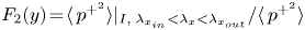${{F}_2}(y) \!=\! \langle \,{p^{{ + ^2}}}\rangle {|_{I,\;{\lambda _{{x_{in}}}} < {\lambda _x} < {\lambda _{{x_{out}}}}}}/ \langle \,{p^{{ + ^2}}}\rangle $,${{F}_3}(y) = \langle \,{p^{{ + ^2}}}\rangle {|_I},{\lambda _x} \ge {\lambda _{{x_{out}}}},{\lambda _z} < {\lambda _{{z_{out}}}}/\langle \,{p^{{ + ^2}}}\rangle$) and large-scale 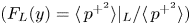$({{F}_{{L}}}(y) = \langle \,{p^{{ + ^2}}}\rangle {|_L}/ \langle \,{p^{{ + ^2}}}\rangle )$ structures defined in § 5.2. However, the relative contribution from the intermediate-scale structures is divided into ${{F}_1}(y)$, ${{F}_2}(y)$ and ${{F}_3}(y)$ as indicated in figure 17(a). With reference to (5.5), the ‘corrected’ convection velocity $c_p^c(\lambda _x^c,y)$ can be indicated as

(5.7) \begin{align} c_p^c(\lambda _x^c,y) & = [{{F}_{{s}}}(y) + {{F}_1}(y)]\; {C}_p^M(y)\notag\\ & \quad + {{F}_2}(y)({A_{{c_p}}}(y)\ln (\lambda _x^{{c^ + }}) + {B_{{c_p}}}(y))\notag\\ & \quad + [{{F}_{{L}}}(y) + {{F}_3}(y)/1.2](0.82{U_{cl}}). \end{align}

The ‘corrected’ scale-dependent convection velocity $c_p^c(\lambda _x^c,y)$ defines a velocity that depends on the streamwise wavelength. It is shown in figure 17(b) for the wall pressure, $c_{{p_w}}^c(\lambda _x^c) = c_p^c(\lambda _x^c,y = 0)$. It simply comprises the convection velocities of the three types of pressure structures in one scale-dependent convection velocity. This convection velocity $c_{{p_w}}^c(\lambda _x^c)$ and its derivative $\textrm{d}c_{{p_w}}^c/\textrm{d}k_x^c$ are continuous. This guarantees, by (5.4), the obtained ‘corrected’ spectrum to be continuous as well. Hence, using a continuous convection velocity is better than using a discontinuous one such that we obtain a continuous spectrum by (5.4).

Figure 17. (a) The relative contributions from the different scales of the pressure structures to the pressure variance. (b) The scale-dependent convection velocity of small-scale $c_{{p_w}}^S(\lambda _x^c) = c_p^S(\lambda _x^c,y = 0)$, intermediate-scale $c_{{p_w}}^I(\lambda _x^c) = c_p^I(\lambda _x^c,y = 0)$ and large-scale 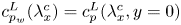$c_{{p_w}}^L(\lambda _x^c) = c_p^L(\lambda _x^c,y = 0)$ structures and the ‘corrected’ scale-dependent convection velocity 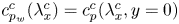$c_{{p_w}}^c(\lambda _x^c) = c_p^c(\lambda _x^c,y = 0)$ for the wall pressure.

The results of the ‘corrected’ spectra are shown for R500 and R2000 for the wall pressure and static pressure at ${y^ + } = 55$ in figures 18(a) and 18(b), respectively, upon applying $c_p^c(\lambda _x^c,y)$. The ‘corrected’ spectra match well the streamwise spectra. The difference between the premultiplied streamwise and ‘corrected’ spectra tends to zero for all streamwise wavelengths except around the peak where it has a maximum value of $O(5\,\%)$.

Figure 18. Same as figures 15 and 16 for R500 and R2000. The ‘corrected’ spectra are computed using the ‘corrected’ convection velocity $c_p^c(\lambda _x^c,y)$ and (5.7).

A note to be mentioned here is that the robustness of the current ‘corrected’ scale-dependent convection velocity $c_p^c(\lambda _x^c,y)$ depends on the convection velocities of the turbulent structures as well as the weights indicated in (5.7). How these weights change across the channel for the different Reynolds numbers is of significance. These details will be reported elsewhere.

6. Conclusion

The first objective of this study was to investigate the convection velocity, as a function of the wall distance, associated with Taylor's hypothesis of the pressure fluctuations based on the comparison between the streamwise wavenumber and Taylor (frequency) spectra. The second objective was to discuss the convection velocity as a function of both scale and wall distance at the wall-normal positions where the difference between both spectra is significant. For such objectives, DNSs of fully developed channel flow of a large computational domain $(25.6h \times 9.6h)$ in the wall-parallel plane were implemented at friction Reynolds numbers of 180, 500 and 2000 based on the channel half-depth h, friction velocity ${u_\tau }$ and kinematic viscosity $\nu $.

The advantage of the current study is that the frozen hypothesis was studied by comparing frequency and streamwise wavenumber spectra from the same DNS database for $R{e_\tau } \le 2000$. Using the local mean velocity for the hypothesis leads to a large difference between both spectra with a value of $O(50\,{\%})$ for its maximum value from the wall to $y/h \approx 0.2$. Alternatively, the convection velocity of the pressure fluctuations, originally defined by Del Álamo & Jiménez (2009) as a function of the wall distance y, is investigated and adopted for the hypothesis. Its value nearly equals the local mean velocity from ${y^ + } = 20$ to the channel centre. From the wall to ${y^ + } = 20$, it is almost constant with a value $12{u_\tau }$ which is equal to the local mean velocity at ${y^ + } = 20$.

This convection velocity can well predict the streamwise spectra from temporal measurements of the pressure field above the wall-normal location $y/h \approx 0.2$. Below that position, the maximum difference between the streamwise and frequency spectra was of $O(10\,\%)$ and it increases with Reynolds number. To address this difference, the pressure field structures were classified into small-, intermediate- and large-scale structures based on the scaling of the premultiplied 2-D spectra. Large-scale structures had length scales larger than h in the wall-parallel plane. Small-scale structures had length scales smaller than the local ridges of the premultiplied 1-D streamwise spectra. Intermediate-scale structures did not qualify as either small or large. The present study verified that intermediate-scale structures are those that mainly dominate the contributions to the pressure variances across the channel. Logarithmic variation of the wall pressure variance with $R{e_\tau }$ as well as logarithmic variation of the static pressure with the distance from the wall are associated with these structures.

Small-scale structures propagated closely with the local mean velocity. Intermediate-scale structures propagated with velocities that depend logarithmically on their size for some range of their length scales. However, this dependence decreased gradually until the convection velocity became consistent with the local mean velocity at $y/h \approx 0.2$. The convection velocity of the large-scale structures approached a constant value of $0.82{U_{cl}}$. Based on the propagation of the three classes of structures, a scale-dependent convection velocity was proposed by weighting the convection velocities of the three classes. The weight functions are the relative contributions of the three classes to the pressure variance. Hence, the obtained spectra from such weighted scale-dependent convection velocity overlap well the wavenumber spectra.