The mean wall-normal velocity in turbulent boundary layer flows under pressure gradient

Abstract

Using a combination of proper variable transformation and integral methods, we rigorously derive an analytical formulation for the mean wall-normal velocity in turbulent boundary layers (TBLs) subjected to arbitrary pressure gradients. The accuracy and robustness of this novel formulation are validated extensively through comparisons with two independent sets of numerical simulation data, demonstrating excellent agreement in both near-equilibrium and non-equilibrium TBLs. In addition, the robustness of the analytical formulations to various choices of boundary-layer edge definition is further confirmed in non-equilibrium TBLs. Our formulation includes a streamwise derivative term, which has minimal significance in near-equilibrium TBLs but plays a crucial role in determining the mean wall-normal velocity in non-equilibrium TBLs. Moreover, we investigate the physical significance of the pre-factors associated with the mean wall-normal velocity components, and unveil a close connection between a previously defined pressure gradient parameter and the ratio of these pre-factors in the analytical equation governing the mean wall-normal velocity. The insights gained from the examination of the pre-factors and their connection to the pressure gradient parameter offer valuable knowledge for interpreting and predicting the behaviour of turbulent boundary layers in various practical applications.

1. Introduction

Turbulent boundary layers (TBLs) play a crucial role in the design and operation of a wide range of practical systems, including aircraft, ships, wind turbines and other fluid systems. A key aspect of understanding TBLs is their behaviour under pressure gradients, as this significantly impacts the performance and energy efficiency of these systems. For instance, under an adverse pressure gradient (APG), the flow within the TBL slows down, and the thickness of the boundary layer increases. In severe cases of APG, the boundary-layer flow may separate from the solid surface, resulting in a drastic change in the flow pattern.

Considerable research efforts have been dedicated to understanding the behaviour of TBLs under pressure gradients through theoretical, experimental and numerical means (Rotta 1950; Clauser 1954; Townsend 1956; Mellor 1966; Mellor & Gibson 1966; Monty, Harun & Marusic 2011; Bobke et al. 2017; Coleman, Rumsey & Spalart 2018; Devenport & Lowe 2022; Subrahmanyam, Cantwell & Alonso 2022). However, previous investigations have concentrated primarily on studying the effects of pressure gradients on the mean streamwise velocity, with relatively less attention given to the behaviour of the mean wall-normal flow. This knowledge gap motivates our present study, where we rigorously derive a novel analytical equation for the mean wall-normal velocity in TBLs subjected to arbitrary pressure gradients.

Experimental measurement of the mean wall-normal velocity $V$ poses significant challenges due to its small magnitude relative to the streamwise velocity. As a result, there is a scarcity of reliable experimental data available for studying $V$. To overcome this limitation and ensure the validity of the derived analytical equation, this study conducts a comprehensive comparison with two independent numerical simulation datasets. The first dataset consists of well-resolved large-eddy simulations (LES) of near-equilibrium APG TBLs conducted by Bobke et al. (2017). The second dataset comprises direct numerical simulations (DNS) of TBLs subjected to first an APG and then a favourable pressure gradient (FPG) (Coleman et al. 2018).

An important challenge in the study of TBLs (particularly when subjected to streamwise pressure gradients) is to determine accurately and consistently the boundary-layer edge (see e.g. Vinuesa et al. 2016; Cantwell 2021; Griffin, Fu & Moin 2021). The conventional approach relies on mean streamwise velocity ($U$) profiles and locates the boundary-layer edge at 99 % of the free-stream velocity (see e.g. Young et al. 2007). However, this method assumes a constant mean streamwise velocity outside the boundary layer, which may not always hold true (see Appendix A for examples). To address this, we adopt a novel method proposed by Wei & Knopp (2023) to determine the boundary-layer edge ($\delta _e$). This method identifies the boundary-layer edge as the location where the Reynolds shear stress decreases to 1 % of its maximum value. Further details about this method can be found in Appendix A. This new approach aligns with the traditional boundary-layer edge determination method when the mean streamwise velocity remains constant outside the boundary layer. The analytical derivation developed in this work is independent of the specific choice of $\delta _e$ and $U_e$. In the main text, the results utilize the $\delta _e$ determined using the new approach. Additionally, in Appendix B, the results obtained using $\delta _e$ defined from the $U$ profiles and diagnostic plot (Vinuesa et al. 2016) are presented for comparison.

Figure 1 illustrates the variation of the mean streamwise velocity at the boundary-layer edge $U_e$ for the two simulations examined in this study. In the well-resolved near-equilibrium flat-plate LES by Bobke et al. (2017), the pressure gradient was imposed through specifying the free-stream velocity at the top of the domain using Townsend's power-law definition (see Townsend 1956; Mellor & Gibson 1966) $C (x-x_0)^m$, where $C$ is a constant, $x_0$ is a virtual origin, and $m$ is the power-law exponent. Five cases of simulations were performed to investigate different near-equilibrium boundary layers by varying the virtual origin and the power-law exponent $m$. These simulations include case m13 ($x_0=60$, $m=-0.13$), case m16 ($x_0=60$, $m=-0.16$), case m18 ($x_0=60$, $m=-0.18$), case b1 ($x_0=100$, $m=-0.14$), and case b2 ($x_0=100$, $m=-0.18$). The lengths in the archived data were normalized by the displacement thickness of the laminar inflow $\delta _1(x_0)$, and the velocities were normalized by the free-stream velocity at the inlet $U_{0}$.

Figure 1. Variation of the mean streamwise velocity at the boundary-layer edge. The ix on the top axis refers to the grid-point number in the $x$-direction. (a) Well-resolved LES of near-equilibrium flat-plate APG TBLs by Bobke et al. (2017). The $x$-location is normalized by the displacement thickness of the laminar inflow $\delta _1(x_0)$. (b) DNS of NEPG TBLs by Coleman et al. (2018). The $x$-location is normalized by the simulation domain height $Y$.

In the DNS of non-equilibrium pressure gradient (NEPG) TBLs by Coleman et al. (2018), pressure gradients were induced by a transpiration profile $V_{top}(x)$ acting through a virtual parallel plane offset a fixed distance $Y$ from the flat no-slip surface. The archived simulation data were normalized by $Y$ and $U_{0}= U_e(x_0)$. Figure 1(b) illustrates that the boundary-layer thickness increases much more rapidly under APG than under zero pressure gradient (ZPG). Although $U_e$ decreases under APG, the product $U_e \delta _e$ increases in the $x$-direction. The maximum value of $U_e \delta _e$ in the APG region is reached near $\mathrm {ix}\approx 4000$. Based on the friction coefficient 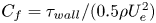$C_f=\tau _{wall}/(0.5 \rho U^2_e)$ data, the TBL separates at $x/Y\approx -1.4$ (${\rm ix} \approx 3500$) and subsequently reattaches at $x/Y \approx 0.4$ (${\rm ix}\approx 4050$). Based on the pressure gradient $\mathrm {d}C_p/\mathrm {d}\kern 0.06em x$ data presented in figure 1(b), it can be determined that the FPG region initiates at approximately ${\rm ix} = 4200$. The pressure coefficient $C_p$ is defined as $C_p = (P-P_\infty )/(0.5 \rho U^2_\infty )$.

Figure 1(b) shows that under FPG, initially $\delta _e$ decreases in the $x$-direction. However, between $\mathrm {ix}\approx 5200$ and $\mathrm {ix}\approx 6000$, the boundary-layer thickness $\delta _e$ increases again, despite the mean pressure gradient being favourable. Similarly, the product $U_e \delta _e$ initially decreases in the FPG region, but then increases again in the $x$-direction. It is important to note that due to the sudden transition from APG to FPG, the FPG region in the DNS may be influenced by the upstream APG effect, especially in the outer region.

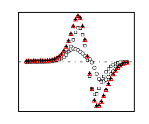
Figure 2 displays the variation of the mean wall-normal velocity at several $x$-stations in the numerical simulations. Under APG, the mean wall-normal velocity is positive and increases linearly outside the boundary layer. On the other hand, under FPG (as seen in the DNS at ${\rm ix} = 5000$), the mean wall-normal velocity is negative, and the boundary-layer thickness decreases in the $x$-direction. Figure 2(b) shows that the mean wall-normal velocity at or near ZPG (${\rm ix} = 1000$ and 6100) is significantly smaller than the mean wall-normal velocity under APG.

Figure 2. Mean wall-normal velocity profiles at different $x$-locations shown in figure 1. (a) Well-resolved LES of near-equilibrium flat-plate APG TBLs by Bobke et al. (2017) (case b1). (b) The DNS of NEPG TBLs by Coleman et al. (2018). The short vertical red line marks the boundary-layer edge.

In this work, we elucidate the characteristics of the wall-normal velocity through an analytical derivation. In § 2, the mean wall-normal velocity at the boundary-layer edge is first derived. An analytical equation for the mean wall-normal velocity is subsequently derived and validated with the numerical simulation data. Section 3 discusses the significance of the components and pre-factors in the analytical equation. Section 4 summarizes the work.

2. Analysis of the mean continuity equation

For a statistically steady two-dimensional TBL under pressure gradient, the mean continuity equation is (see e.g. Tennekes & Lumley 1972)

(2.1)\begin{equation} 0 = \frac{\partial U}{\partial x} + \frac{\partial {V}}{\partial y}, \end{equation}

where the upper-case letters $U$ and $V$ represent the mean velocity component in the streamwise ($x$) and wall-normal ($y$) directions, respectively. In order to derive an analytical equation for the mean wall-normal velocity $V$, we first transform the mean continuity equation into a dimensionless form. To achieve this, we define the normalized variables

(2.2a–d)

where $L$ is a length scale in the $x$-direction. While normalized streamwise velocity can also be $U/U_e$, in this work, we define $U^-$ as $1-U/U_e$ for a bounded integral $\int _0^\infty U^-\, \mathrm {d}y^-$. It is important to emphasize that this normalization does not assume any self-similarity of $U^-$ or $V^-$.

Using the defined normalized variables, the terms in the mean continuity equation can be written as

(2.3)\begin{equation} \left.\begin{gathered} \frac{\partial U}{\partial x} = \frac{\mathrm{d} U_e}{\mathrm{d}\kern 0.06em x} - \frac{\mathrm{d} U_e}{\mathrm{d}\kern 0.06em x}\,U^-{-} \frac{U_e}{L}\,\frac{\partial U^-}{\partial x^*} + \frac{U_e}{\delta_e}\,\frac{\mathrm{d} \delta_e}{\mathrm{d}\kern 0.06em x}\,y^-\, \frac{\partial U^-}{\partial y^-}, \\ \frac{\partial V}{\partial y} = \frac{|V_e|}{\delta_e}\,\frac{\partial V^-}{\partial y^-}. \end{gathered}\right\} \end{equation}

Simple mathematics produces a dimensionless continuity equation in the form

(2.4)\begin{equation} 0 = \frac{\delta_e}{|V_e|}\,\frac{\mathrm{d} U_e}{\mathrm{d}\kern 0.06em x}- \frac{1}{|V_e|}\,\frac{\mathrm{d} (U_e \delta_e)}{\mathrm{d}\kern 0.06em x}\,U^-{+} \frac{U_e}{|V_e|}\,\frac{\mathrm{d} \delta_e}{\mathrm{d}\kern 0.06em x}\, \frac{\partial (y^- U^-)}{\partial y^-} - \frac{U_e}{|V_e|}\,\frac{\delta_e}{L}\,\frac{\partial U^-}{\partial x^*} + \frac{\partial V^-}{\partial y^-}. \end{equation}

2.1. Mean wall-normal velocity at the boundary-layer edge

The mean wall-normal velocity $V_e$ at the edge of the boundary layer can be obtained by performing integration of (2.4) with respect to $y^-$ from the wall $y^-=0$ to the boundary-layer edge $y^-=1$:

(2.5)\begin{equation} V_e ={-} {\delta_e}\,\frac{\mathrm{d} U_e}{\mathrm{d}\kern 0.06em x} + \frac{\mathrm{d} (U_e\delta_e)}{\mathrm{d}\kern 0.06em x}\, \frac{\delta_1}{\delta_e} + U_e\,\frac{\delta_e}{L} \int_0^1 \frac{\partial U^-}{\partial x^*}\,\mathrm{d}y^-. \end{equation}

Note that by definition, $\int _0^{1} U^-\,\mathrm {d}y^- =\delta _1/\delta _e$, where $\delta _1$ is the mass displacement thickness (see Schlichting 1979). In a ZPG TBL, the mean streamwise velocity beyond the boundary-layer edge $\delta _e$ remains constant in the wall-normal $y$-direction. However, when a TBL is subjected to a pressure gradient, the mean streamwise velocity beyond $\delta _e$ may vary in the $y$-direction (see Appendix A). The evaluation of the last term in (2.5) involves absorbing the length scale $L$ back into $x^*$. As a result, the specific choice of $L$ becomes inconsequential to the evaluation.

Figure 3 illustrates the simulation data for $V_e$, accompanied by the three terms on the right-hand side of (2.5), as well as their sum. The simulation data exhibit excellent agreement with the analytical equation (2.5). In figure 3(a), it is evident that the term involving $\partial U^-/\partial x^*$ is relatively small within the near-equilibrium APG TBL ($1000 < x/\delta _1(x_0) < 2200$), and its contribution can be considered negligible in such situations. However, as shown in figure 3(b), the term involving $\partial U^-/\partial x^*$ becomes significant when the TBL undergoes rapid changes in pressure gradient, and cannot be neglected.

Figure 3. Comparison of simulation data of $V_e$ with (2.5). (a) Case b1 from the LES of Bobke et al. (2017). (b) The DNS of Coleman et al. (2018). To prevent clutter, every 100th grid in the $x$-direction is plotted. Markers for $V_e$ represent values obtained directly from simulation data, while the sum is calculated from terms on the right-hand side of (2.5).

By applying the Leibniz integral rule to the last term in (2.5), the mean wall-normal velocity at the boundary-layer edge can be simplified as

(2.6)\begin{equation} V_e ={-} {\delta_e}\,\frac{\mathrm{d} U_e}{\mathrm{d}\kern 0.06em x} + \frac{\mathrm{d} (U_e\delta_1)}{\mathrm{d}\kern 0.06em x}. \end{equation}

For a ZPG boundary layer, where $U_e$ remains constant, (2.6) can be simplified further to $V_e=U_e\, \,\mathrm {d}\delta _1/\mathrm {d}\kern 0.06em x$, as reported by Wei, Li & Wang (2023a).

It is intriguing to observe that the functional form of (2.6) exhibits certain similarities to Kármán's integral equation $u^2_\tau = (U_e \delta _1)\,{\mathrm {d}U_e}/{\mathrm {d}\kern 0.06em x} + {\mathrm {d}(U^2_e \delta _2)}/{\mathrm {d}\kern 0.06em x}$. Kármán's integral equation is derived by integrating globally both the mean continuity and momentum equations (see e.g. Schlichting 1979). Equation (2.6) is also valid for the laminar (Falkner–Skan) case, as it is derived solely from the continuity equation without making any assumptions about turbulence or pressure gradients.

Figure 4 illustrates the simulation data of $V_e$, along with the two terms on the right-hand side of (2.6), and their sum. The mean wall-normal velocity magnitude is observed to be significantly higher under APG or FPG as compared to ZPG. This amplified wall-normal convection in the APG TBL has been reported in simulations of TBLs around wing sections (Vinuesa et al. 2018). Figure 4 demonstrates that the sum of the terms on the right-hand side of (2.6) exhibits better agreement with the directly simulated $V_e$ in comparison to the sum of the terms on the right-hand side of (2.5). Mathematically, (2.5) and (2.6) are equivalent. The enhanced accuracy observed in the post-processing with (2.6) can be attributed to its improved precision in calculating the $x$-derivative from $\delta _1$, which represents an integral quantity. In Appendix B, we demonstrate that the validity of (2.6) is independent of the method used to determine the boundary-layer edge (see figure 18).

Figure 4. Comparison of simulation data of $V_e$ with (2.6). (a) Case b1 from the LES of Bobke et al. (2017). (b) The DNS of Coleman et al. (2018). To prevent clutter, every 100th grid in the $x$-direction is plotted. Markers for $V_e$ represent values obtained directly from simulation data, while the sum is calculated from terms on the right-hand side of (2.6).

Figure 4 shows that in APG TBLs, both terms on the right-hand side of (2.6) are positive, and $V_e$ is also positive, resulting in the rapid growth of the boundary layer. Conversely, under FPG, $U_e$ increases in the $x$-direction, and as shown in figure 4(b), the first term on the right-hand side of (2.6) becomes negative.

2.2. Analytical equation for $V$

Integrating (2.4) with respect to $y^-$ yields an analytical equation for the mean wall-normal velocity distribution:

(2.7) \begin{align} V^- &= \underbrace{-\frac{\delta_e}{|V_e|}\, \frac{\mathrm{d} U_e}{{\mathrm{d}}\kern 0.06em x}}_{a_{I}}\,y^- \underbrace{{}-\frac{U_e}{|V_e|}\,\frac{\mathrm{d} \delta_e}{\mathrm{d}\kern 0.06em x}}_{a_{II}}\,y^- U^-{+} \underbrace{\frac{1}{|V_e|}\,\frac{{\mathrm{d}} (U_e\delta_e)}{{\mathrm{d}}\kern 0.06em x}}_{-(a_{I}+a_{II})} \int_0^{y^-} U^-\,\mathrm{d}y^- \nonumber\\ &\quad + \underbrace{\frac{U_e}{|V_e|}\, \frac{\delta_e}{L}}_{a_{III}} \int_0^{y^-} \frac{\partial U^-}{\partial x^*}\, \mathrm{d}y^-. \end{align}

For a constant value of $U_e$, (2.7) simplifies to $V^-=(U_e/|V_e|)\,\mathrm {d}\delta _e/\mathrm {d}\kern 0.06em x (-y^-U^- + \int _0^{y^-}$ $U^-\,{\textrm {d}y}^-) + (U_e/|V_e|)(\delta _e/L)\int _0^{y^-}(\partial U^-/\partial x^*)\,{\textrm {d}y}^-$, as reported by Wei et al. (2023a) for the normalized mean wall-normal velocity in a ZPG boundary layer.

To illustrate the four components of the mean wall-normal velocity in an APG TBL, figure 5 uses the well-resolved LES data of near-equilibrium APG TBLs by Bobke et al. (2017). Under an APG, $U_e$ experience a decrease while $\delta _e$ increases in the $x$-direction. As a result, $a_{I}$ is positive and $a_{II}$ is negative.

Figure 5. Illustration of the four components in (2.7) for an APG TBL. The data are from the well-resolved LES data of near-equilibrium APG TBLs by Bobke et al. (2017): case b1 at the 1000th grid point in $x$.

Figure 6 shows the different components of the mean wall-normal velocity under transition from APG to FPG, as obtained from the DNS of Coleman et al. (2018). In the APG section, the first, second and third terms in the DNS data behave similarly to those shown in figure 5. However, the last term with $x$-derivative has a significantly larger magnitude in the DNS data, indicating that the TBL is not in a near-equilibrium state. In the FPG section, the first and last terms of (2.7) are negative, as shown in figure 6(b).

Figure 6. Wall-normal velocity and its components from the DNS data of NEPG TBLs by Coleman et al. (2018). (a) The APG section at $\textrm {ix} = 2800$. (b) The FPG section at $\textrm {ix} = 5000$.

To provide further validation of (2.7), the mean wall-normal velocity profiles at various $x$-stations presented in figure 2 are normalized and compared with the analytical equation in figure 7. The figure demonstrates the excellent agreement between the simulation data and the analytical equation. In Appendix B, we demonstrate that the accuracy of (2.7) is not affected by the method used to determine the boundary-layer edge (see figure 20). The shapes of the $V/|V_e|$ versus $y/\delta _e$ profiles, however, may vary due to the use of different methods for determining the boundary-layer edge and the resulting differences in $\delta _e$ and $V_e$ values (see Appendix B).

Figure 7. Normalized $V/|V_e|$ obtained directly from simulation data (open symbols) and the sum of terms on the right-hand side of (2.7) (filled symbols) plotted against $y/\delta _e$. (a) Well-resolved LES data of near-equilibrium APG TBLs by Bobke et al. (2017). (b) The DNS data of NEPG TBLs by Coleman et al. (2018).

In ZPG TBL, $V^-$ is approximately a self-similar function of $y^-$, as observed by Wei & Klewicki (2016). However, in TBL under pressure gradient, especially when the pressure gradient varies over a short distance, the mean wall-normal velocity profile undergoes a rapid change in shape and magnitude. Figure 8 presents the mean wall-normal velocity profiles around the location where the pressure gradient switches from APG to FPG. In figure 8(a), the raw data show a smaller magnitude of $V$ (magnitude of 0.02 in figure 8(a) versus 0.1 in figure 2(b)), and a change of velocity direction. Moreover, the shapes of the mean wall-normal velocity at the three stations are distinctively different. In figure 8(b), the mean wall-normal velocity normalized by $|V_e|$ is presented. While the analytical equation captures the general trend of $V$, there are noticeable deviations at stations $\textrm {ix} = 3900$ and 4000. These deviations can be attributed to the rapid shift from APG to FPG, which amplifies the numerical errors in the finite-difference calculation of ${\partial U^-}/\partial x^*$ in (2.7) at $\textrm {ix} = 3900$ and 4000.

Figure 8. Plots of $V$ profiles from DNS data of NEPG TBLs by Coleman et al. (2018) at three different locations near $x/Y=0$: (a) raw data, (b) normalized data.

3. Discussion

The analytical equation (2.7) provides valuable insights into the composition of the mean wall-normal velocity in TBLs under arbitrary pressure gradients. It reveals that the mean wall-normal velocity can be decomposed into four distinct components, as depicted in figures 5 and 6. It is interesting to note that the first three components in (2.7) for the mean wall-normal velocity in the TBL bear a strong resemblance to those observed for the mean transverse flow in planar turbulent wakes under pressure gradients, as discussed in Wei et al. (2023b).

The parameters $a_{I}$, $a_{II}$, $-(a_{I}+a_{II})$ and $a_{III}$ in (2.7) represent the ratios of the characteristic velocity for each component to $|V_e|$. Figure 9 illustrates the variations of these parameters with $x$-locations. In near-equilibrium APG TBLs, $a_{I}$ is approximately 0.5, and $a_{II}$ is negative with magnitude approximately 2. In the DNS of TBL under rapid changes between APG and FPG, $a_{I}$ varies between $-1$ and 1. The magnitudes of $a_{II}$ and $-(a_{I}+a_{II})$ are approximately 1, except near the leading and trailing edges of the domain.

Figure 9. Pre-factors of the three terms on the right-hand side of (2.7). (a) Well-resolved LES of near-equilibrium APG TBL by Bobke et al. (2017). (b) The DNS of NEPG TBLs by Coleman et al. (2018). To prevent clutter, only every 100th grid in $x$ is plotted.

The first term on the right-hand side of (2.7) is a linear function of $y$, and is associated with the imposed pressure gradient $-\mathrm {d} (P_e/\rho )/\mathrm {d}\kern 0.06em x$ or $U_e \,\mathrm {d} U_e/\mathrm {d}\kern 0.06em x$. In an APG (FPG) TBL, the parameter $a_{I}$ is positive (negative) due to the sign of $\mathrm {d} U_e/\mathrm {d}\kern 0.05em x$. Additionally, $a_{I}$ can also be expressed as

(3.1)\begin{equation} a_{I} ={-}\frac{\delta_e}{|V_e|}\,\frac{\mathrm{d} U_e}{\mathrm{d}\kern 0.06em x} = \frac{\left.\dfrac{\partial V}{\partial y}\right|_{e}}{\dfrac{|V_e|}{\delta_e}}. \end{equation}

The parameter $a_{I}$ can therefore be interpreted as the ratio of two slopes, namely the slope $\partial V/\partial y|_e$ of the mean wall-normal velocity profile at the boundary-layer edge, and the slope of $|V_e|/\delta _e$. This relationship is illustrated in figure 10, where the normalized mean wall-normal velocity $V/V_e$ is plotted against the normalized wall-normal distance $y/ \delta _e$. In the case of an APG TBL, where $V_e$ is positive, this figure is equivalent to figure 6(a). On the other hand, in an FPG TBL where $V_e$ is negative, figure 10 is analogous to vertically flipping figure 6(b) onto the positive side.

Figure 10. Visual representation of terms in (2.6) for $V/|V_e|$.

Figure 11 illustrates the impact of pressure gradient on the ratio of the two terms on the right-hand side of (2.6), as shown in figure 10. In the ZPG TBL, the ratio is zero since $\mathrm {d}U_e/\mathrm {d}\kern 0.06em x=0$. In the near-equilibrium APG TBL, as observed in figure 11(a), the ratio remains nearly constant at 1. For the FPG TBL, both $\delta _e$ and $\delta _1$ decrease in the $x$-direction, indicating a thinner boundary layer. In the non-equilibrium TBL simulated by Coleman et al. (2018), the product $U_e \delta _1$ initially decreases in the FPG TBL region and then increases towards the end of the simulation domain. Consequently, in the FPG region of the DNS data, the ratio can be either positive or negative, and its magnitude can exceed 1 significantly.

Figure 11. Ratio of the two terms on the right-hand side of (2.6). (a) Well-resolved LES of APG TBLs by Bobke et al. (2017). (b) The DNS of NEPG TBLs by Coleman et al. (2018).

The ratio between $a_{I}$ and $a_{II}$ is equivalent to the pressure gradient parameter $\varLambda$ defined by Castillo & George (2001), with the only difference being a negative sign:

(3.2)\begin{equation} \frac{a_{I}}{a_{II}} = \frac{\delta_e\,\dfrac{\mathrm{d} U_e}{\mathrm{d}\kern 0.06em x}}{U_e\, \dfrac{\mathrm{d} \delta_e}{\mathrm{d}\kern 0.06em x}} ={-} \varLambda. \end{equation}

From their analysis of experimental data, Castillo & George (2001) reported that the pressure gradient parameter $\varLambda$ is approximately $0.22$ for APG TBLs, and $-1.92$ for FPG TBLs. However, the universality of these values has been a topic of debate, as pointed out by Maciel, Rossignol & Lemay (2006).

In near-equilibrium APG TBLs, the last term on the right-hand side of (2.5) is negligible. Additionally, as illustrated in figure 12, the ratio of $-\delta _e \,{\mathrm {d} U_e}/{\mathrm {d}\kern 0.06em x}$ to $({\delta _1}/{\delta _e})\,{\mathrm {d} (U_e \delta _e)}/{\mathrm {d}\kern 0.06em x}$ is approximately $1$ within the region $1000 \lesssim x/\delta _1({x_0}) \lesssim 2200$. Setting the ratio in figure 12 to be 1, the pressure gradient parameter defined by Castillo & George (2001) can be approximated as

(3.3)\begin{equation} \varLambda ={-} \frac{a_{I}}{a_{II}} = \frac{-\delta_e\,\dfrac{\mathrm{d} U_e}{\mathrm{d}\kern 0.06em x}}{U_e\, \dfrac{\mathrm{d} \delta_e}{\mathrm{d}\kern 0.06em x}} \approx \frac{1}{1 + \dfrac{\delta_e}{\delta_1}}\quad (\text{near-equilibrium APG TBL}). \end{equation}

Figure 12. Ratio of $-\delta _e ({\mathrm {d} U_e}/{\mathrm {d}\kern 0.06em x})$ to $({\mathrm {d} (U_e \delta _e)}/{\mathrm {d}\kern 0.06em x}) ({\delta _1}/{\delta _e})$. Data are from the well-resolved LES of near-equilibrium APG TBLs by Bobke et al. (2017).

Figure 13 compares the approximation (3.3) with experimental and LES data. While both the experimental and LES data show that $\varLambda$ is not constant, they agree well with the predicted trend given by (3.3).

Figure 13. (a) Comparison of the approximate (3.3) and experimental data of Skåre & Krogstad (1994). The $x$-location is normalized by the boundary-layer thickness at the first measurement station. (b) Comparison of the approximate (3.3) and well-resolved LES data of near-equilibrium APG TBLs by Bobke et al. (2017).

Figure 14(a) shows the ratio of the first two terms in (2.5) for $V_e$ from the DNS data of NEPG TBLs by Coleman et al. (2018). The ratio is approximately $1$ over a short distance within the APG region, and $\varLambda$ is close to the value $0.22$ suggested for the near-equilibrium APG TBLs, as shown in figure 14(b). However, it is important to note that $\varLambda$ is not constant from the leading edge to the end of the APG region, but exhibits a smooth variation. As shown in figure 14(b), the approximation in (3.3) works well for estimating $\varLambda$ in the APG TBL when it is in a near-equilibrium state. However, this approximation is not valid for FPG TBLs.

Figure 14. (a) Ratio of the first two terms on the right-hand side of (2.5) for $V_e$. (b) Plots of $\varLambda = -a_{I}/a_{II}$ and DNS data of NEPG TBLs by Coleman et al. (2018).

The variation of $\varLambda$ in the region $0 \lesssim x/Y \lesssim 7$ is more complicated. For $0 \lesssim x/Y \lesssim 4$, where a strong FPG is present, $U_e$ increases while $\delta _e$ decreases in the $x$-direction. As a result, $a_{I}$ becomes negative, $a_{II}$ becomes positive, and $\varLambda$ becomes positive. However, at approximately $x/Y=5$, $\mathrm {d} \delta _e/\mathrm {d}\kern 0.06em x \approx 0$ (see figure 1b), causing $\varLambda$ to diverge to infinity. Beyond this point, i.e. for $x/Y \gtrsim 5$, $\delta _e$ begins to increase in the $x$-direction, despite the presence of a weak FPG. This results in a negative value of $\varLambda$.

The right-hand side of (3.3), computed from an integral quantity $\delta _1$, provides greater numerical robustness and consistent values. It is close to the value suggested by Castillo & George (2001) for near-equilibrium flow conditions (figure 13b). Even in the non-equilibrium flow studied by Coleman et al. (2018), the approximation remains almost constant in the first part of the APG region sufficiently upstream of separation. In accordance with Wei & Knopp (2023), $\delta _1$ corresponds to the wall distance $y_{m}$ of maximum Reynolds shear stress. In flows approaching equilibrium, the position of $y_{m}$ undergoes minimal changes.

4. Summary

This study investigates the behaviour of the mean wall-normal velocity in turbulent boundary layers (TBLs) subjected to pressure gradients. Through rigorous derivation, new analytical equations are developed to describe accurately the distribution of the mean wall-normal velocity and its value at the boundary-layer edge. These analytical equations are validated thoroughly against two independent numerical simulation datasets, demonstrating excellent agreement. Importantly, the evaluation of the simulation data highlights the robustness of the derived equations, confirming their independence from the specific method used to determine the boundary-layer edge.

The analytical equation for the mean wall-normal velocity is decomposed into four components, with only one of them involving the streamwise derivative of the $U$ profile. In near-equilibrium TBLs, this component is found to be negligible, while in non-equilibrium cases, it plays a significant role. Furthermore, this study explores the characteristics of the pre-factors in the analytical equation for the mean wall-normal velocity, and establishes a close connection between the ratio of these pre-factors and a pressure-gradient parameter defined previously in the literature. By bridging an existing gap in the literature, this analysis enhances our understanding of the behaviour of TBLs under pressure gradients, contributing to more comprehensive knowledge in this field. Overall, this work represents a significant advancement in our knowledge of TBLs, and provides valuable insights for the analysis and prediction of mean wall-normal velocity profiles in such flows.