


1. Introduction
Wall-bounded turbulent flows subject to rotation are important in terms of engineering (Jiménez Reference Jiménez2011; Jing & Ducoin Reference Jing and Ducoin2020). When rotation is coupled to the wall-bound turbulence as a body force, the near-wall dynamics is different from those in traditional boundary layers (Jiménez & Pinelli Reference Jiménez and Pinelli1999).
The study of rotation in wall-bound turbulence began with experiments of the spanwise-rotating channel (Johnston, Halleent & Lezius Reference Johnston, Halleent and Lezius1972). In channel turbulence with spanwise rotation, the symmetry in the wall-normal direction is broken (Kristoffersen & Andersson Reference Kristoffersen and Andersson1993). Oberlack (Reference Oberlack2001) used group analyses to deduce the linear profiles of the mean velocity. The linear profiles and related scaling laws were further discussed by Xia, Shi & Chen (Reference Xia, Shi and Chen2016). Additionally, couples of Taylor–Görtler-like (TGL) vortices were found in spanwise-rotating channel turbulence (Dai, Huang & Xu Reference Dai, Huang and Xu2016). Brethouwer (Reference Brethouwer2017) found that the intensity and size of the TGL vortices decrease at high rotation rates. In streamwise-rotating channel turbulence the symmetry is still conserved (Oberlack, Cabot & Rogers Reference Oberlack, Cabot and Rogers1999). However, a secondary mean flow, i.e. a mean flow perpendicular to the streamwise direction, is induced by streamwise rotation (Wu & Kasagi Reference Wu and Kasagi2004; Dai, Huang & Xu Reference Dai, Huang and Xu2019). The secondary flow is inverted around the channel centre (Yang, Su & Wu Reference Yang, Su and Wu2010). Such an inverse secondary mean flow has not been observed in experiments due to the measurement accuracy (Recktenwald et al. Reference Recktenwald, Weller, Schröder and Oberlack2007; Alkishriwi, Meinke & Schröder Reference Alkishriwi, Meinke and Schröder2008; Recktenwald, Alkishriwi & Schröder Reference Recktenwald, Alkishriwi and Schröder2009). However, Oberlack et al. (Reference Oberlack, Cabot, Pettersson Reif and Weller2006) used group analyses to analytically study streamwise-rotating channel turbulence and qualitatively found the existence of the inverse secondary mean flow. Masuda, Fukuda & Nagata (Reference Masuda, Fukuda and Nagata2008) further verified this through instability analysis. Yang et al. (Reference Yang, Su and Wu2010) used helical wave decomposition to deduce the inviscid inertial wave solution, which gave a trigonometric profile. This prediction is suitable for the spanwise mean velocity in the bulk region but is not reasonable for the streamwise mean velocity due to the possible effects of the external mean pressure gradient. Yang et al. (Reference Yang, Deng, Wang and Shen2020a) studied the non-monotonic tendency of the spanwise mean velocity with increasing rotation rates and attributed it to the self-constraint mechanism of the Reynolds stress  $\langle u_2u_3 \rangle$. Yang et al. (Reference Yang, Deng, Wang and Shen2018) discussed the pressure fluctuations in this flow. Additionally, since streamwise-rotating channel turbulence is a typical chirality-asymmetric flow, helicity (
 $H=\boldsymbol {u}\boldsymbol {\cdot } \boldsymbol {\omega }$) is also an important quantity here. Recently, Yu et al. (Reference Yu, Hu, Yan and Li2022) and Yan, Li & Yu (Reference Yan, Li and Yu2022) discussed the distribution and budget balance of the helicity in streamwise-rotating channel turbulence. In terms of coherent structures, Yang et al. (Reference Yang, Su and Wu2010) found that when the rotation number
  $Ro_\tau =30$, the inclined vortex columns moving downstream are likely the carriers of inertial waves. Yang & Wang (Reference Yang and Wang2018) found that TGL vortices exist when
  $Ro_\tau =150$. These TGL vortices have negligible inclination angles and are almost aligned with the rotation axis
  $x_1$. Their spanwise length scale is independent of
  $Ro_\tau$, but their streamwise length scale exhibits a considerable dependence on
  $Ro_\tau$ (Yang & Wang Reference Yang and Wang2018). Dai et al. (Reference Dai, Huang and Xu2019) studied the coherent structures in the streamwise-rotating channel through direct numerical simulations (DNS) and large eddy simulations. They found that the elongated streamwise vortices are tilted toward the spanwise direction, and the inclination angle initially increases and then decreases with increasing rotation rates. However, the mechanisms for this non-monotonic tendency are still not clear.
Turbulence is in fact a multiscale physical problem. To study the interscale dynamics, various approaches have been applied by researchers (Lumley Reference Lumley1964; Danaila et al. Reference Danaila, Anselmet, Zhou and Antonia2001; Dunn & Morrison Reference Dunn and Morrison2003). Utilizing the Fourier transform, Lumley (Reference Lumley1964) first derived the spectral energy equation for the interscale energy transfer. Bolotnov et al. (Reference Bolotnov, Lahey, Drew, Jansen and Oberai2010) statistically studied the interscale energy transfer in channel turbulence with a low Reynolds number. Dunn & Morrison (Reference Dunn and Morrison2003) used orthogonal wavelets to analyse spatial and interscale (both forward and backward) energy transfers. However, these approaches do not allow for a distinction between spatial and interscale transfers in the wall-normal direction, which can be addressed using the second-order structure function and its budget balance (Cimarelli et al. Reference Cimarelli, De Angelis, Jimenez and Casciola2016; Mizuno Reference Mizuno2016). The second-order structure function has been used by Kolmogorov (Reference Kolmogorov1941) to study the energy cascades in homogeneous isotropic turbulence, and its evolution equation is known as the Kolmogorov equation. The second-order structure function can be interpreted as the amount of energy of a given scale at a certain position and is also called the scale energy (Marati, Casciola & Piva Reference Marati, Casciola and Piva2004; Cimarelli et al. Reference Cimarelli, De Angelis, Schlatter, Brethouwer, Talamelli and Casciola2015, Reference Cimarelli, De Angelis, Jimenez and Casciola2016). The approach was first generalized to channel turbulence by Danaila et al. (Reference Danaila, Anselmet, Zhou and Antonia2001) and further extended to general flows by Hill (Reference Hill2002). In these flows, the extended budget equation is called the generalized Kolmogorov equation (GKE). Then, the GKE was used to study the energy cascades in channel turbulence by Marati et al. (Reference Marati, Casciola and Piva2004). Based on the GKE, Cimarelli, De Angelis & Casciola (Reference Cimarelli, De Angelis and Casciola2013) found the near-wall turbulence regeneration cycle and the outer self-sustaining mechanism in channel turbulence. Cimarelli et al. (Reference Cimarelli, De Angelis, Schlatter, Brethouwer, Talamelli and Casciola2015) found that the energy source in the outer layer modifies nearby energy fluxes and then affects the energy transfers in the vicinity of the wall. Cimarelli et al. (Reference Cimarelli, De Angelis, Jimenez and Casciola2016) further used the GKE to study the interscale energy transfer in the wall-normal direction and found two ways of interscale energy transfer, consistent with the classical attached vortex model (Marusic & Monty Reference Marusic and Monty2019). The GKE has also been used to study the dynamics in flows with separation and reattachment (Mollicone et al. Reference Mollicone, Battista, Gualtieri and Casciola2018). The anisotropic generalized Kolmogorov equation (AGKE), i.e. the budget equation for the second-order structure function of Reynolds stresses, was first investigated by Gatti et al. (Reference Gatti, Chiarini, Cimarelli and Quadrio2020), who took more details of the interscale dynamics into consideration. Notably, even if the scale energy is strictly related to the energy spectra, it is not an intensive quantity (Cimarelli et al. Reference Cimarelli, De Angelis, Schlatter, Brethouwer, Talamelli and Casciola2015). At small scales, the scale energy could be approximately treated as the eddy intensity of these scales. However, this interpretation is not suitable when the separation is sufficiently large. In fact, as the scale tends to be infinite, the scale energy is reduced to four times the turbulence kinetic energy (TKE) (Marati et al. Reference Marati, Casciola and Piva2004). Yang et al. (Reference Yang, Su and Wu2010) used helical wave decomposition to investigate the interscale dynamics in streamwise-rotating channel turbulence. However, this approach cannot give the spatial-local interscale dynamics, such as the near-wall dynamics. Yang et al. (Reference Yang, Deng, Wang and Shen2020b) took the interscale transfer into consideration via the budget balance for the spectral TKE. They discussed the sustaining mechanisms of the TGL vortices and found that four key processes are responsible for sustaining the motion of large-scale TGL vortices.
In summary, in streamwise-rotating channel turbulence, the study of near-wall multiscale dynamics under moderate rotation rates is still insufficient. This paper focuses on the coupling effects of moderate rotation and boundary layers on turbulence. Specifically, basic turbulence statistics are first examined, where we find the scale discrepancy of inclined structures. To be more concrete, the scale discrepancy is further identified using the newly defined angle based on the velocity vector. The focus then shifts to the sustaining mechanisms of the inclined structures. Several key terms in the Reynolds stress budget balance are identified, and corresponding physical processes are illustrated through ejections and sweeps in the hairpin vortex model. Finally, a mechanism responsible for the scale discrepancies is given utilizing the AGKE.
The paper is organized as follows. We give the details of the simulations and basic statistics in § 2. Next, in § 3 we analyse the basic interscale dynamics through the scale energy and GKE. Section 4 gives the main results of this paper, where we identify the multiscale inclined structures and their sustaining mechanisms. Finally, conclusions are given in § 5.
2. Numerical simulations
2.1. Numerical set-up
The incompressible Navier–Stokes equations are
 \begin{equation} \left. \begin{array}{c} \displaystyle \dfrac{\partial { U_i}}{\partial t} +{ U_j} \dfrac{\partial U_i}{\partial x_j} ={-}\dfrac{1}{\rho}\dfrac{\partial p}{\partial x_i} +\nu \dfrac{\partial^2 U_i}{\partial x_j\partial x_j} +2 \epsilon_{ij1}{ U_j }\varOmega-\dfrac{\varPi_0}{\rho}\delta_{i1}, \\ \displaystyle \dfrac{\partial U_i}{\partial x_i} =0, \end{array}\right\} \end{equation}
where  $U_i$ is the velocity,
  $p$ is the total pressure including the centrifugal effects (Davidson Reference Davidson2013),
  $\rho$ is the density,
  $\nu$ is the kinematic viscosity,
  $\varOmega$ is the rotation rate in the streamwise direction,
  $\varPi _0$ is a constant streamwise pressure gradient that drives the flow,
  $\delta _{ij}$ is the Kronecker delta and
  $\epsilon _{ijk}$ is the Levi-Civita symbol. Equation (2.1) is solved through a pseudo-spectral code using Fourier series in the streamwise and spanwise directions and Chebyshev polynomials in the wall-normal direction. The 3/2 rule is utilized to remove aliasing errors. A third-order time-splitting method is used for time advancement. More details can be found in previous works (Deng & Xu Reference Deng and Xu2012; Yang & Wang Reference Yang and Wang2018). A sketch of the computational configuration and the mean velocities is given in figure 1.

Figure 1. Sketch of the streamwise-rotating channel turbulence. The red and blue lines are the mean velocity profiles.
There are two non-dimensional parameters based on the friction velocity, i.e. the Reynolds and rotation numbers
 \begin{equation} Re_\tau=u_\tau h/\nu, \quad Ro_\tau=2\varOmega h/u_\tau, \end{equation}
where  $u_\tau$ is the friction velocity and
  $h=1$ is the channel half-width. In addition, the friction velocity
  $u_\tau$ and the viscous length scale
  $\nu /u_\tau$ are used to normalize the quantities in the following analyses, which are marked by the superscript ‘
 $+$’. Our DNS data include five cases, in which
  $Ro_\tau$ ranges from
  $0$ to
  $60$ and
  $Re_\tau = 180$ or
  $395$. Except for ST30S and ST60S, the computational domains of the cases are selected based on the third criterion of Yang & Wang (Reference Yang and Wang2018), which has been verified by Yu et al. (Reference Yu, Hu, Yan and Li2022). Cases ST30S and ST60S have relatively small streamwise sizes. The data used in this paper are time averaged over 40
  $h/u_\tau$ after reaching the statistical steady state. As verified through the approach of Russo & Luchini (Reference Russo and Luchini2017), the time slices are independent of each other. The relative standard deviation of the data is less than
  $1\,\%$. In addition, the reliability of the data can also be confirmed through the balance of the budget equation in the following analysis. The parameters are summarized in table 1.
Table 1. Computational descriptions of simulations.

2.2. Basic turbulence statistics
Figure 2 gives the profiles of mean velocities  $\langle U_1 \rangle ^+$ and
  $\langle U_3 \rangle ^+$, where
  $\langle {\cdot } \rangle$ represents averaging over time and the
  $x_1-x_3$ plane. In the following analysis, if the non-dimensional wall-normal coordinates (
 $x_2^+$) are used, then the data in the upper domain (
 $x_2\in [0,1]$) are discussed by default. The black dashed lines in figure 2(a) represent the linear law and log law with the Kármán constant
  $\kappa =0.4$. The black dashed lines in figure 2(b) indicate the linear law with an amplitude of
  $0.18$ as well as the trigonometric function
  $A\sin (2{\rm \pi} f (x_2^+-180))$ with
  $f=1/169.7$ and
  $A=0.17$. As shown in figure 2, ST30 and ST30S have the same mean velocity profile. It will also be shown in § 3.1 that the second-order structure functions of the two cases are also nearly identical. Since the streamwise size of ST60S increases by the same ratio of
  $Ro_\tau$ compared with ST30S, ST60S can at least provide reliable basic statistics. As shown in figure 2(a), rotation does not affect the linear law of
  $\langle U_1 \rangle ^+$ in the viscous sublayer. In the log-law layer the profile of
  $\langle U_1 \rangle ^+$ is still logarithmic, while the amplitudes are suppressed by rotation. In figure 2(b) the spanwise mean velocity
  $\langle U_3 \rangle ^+$ is induced by rotation. In the bulk region,
  $\langle U_3 \rangle^+$ is reversed and has a trigonometric profile, which is the inviscid inertial wave solution of streamwise-rotating channel turbulence (Yang et al. Reference Yang, Su and Wu2010). Furthermore,
  $\langle U_3 \rangle ^+$ in the viscous sublayer has a linear profile, which is also confirmed in the inset of figure 2(b). Up to rotation number
  $Ro_\tau =30$, the stronger the rotation is, the faster
  $\langle U_3 \rangle ^+$ increases. However, the tendency is reversed as
  $Ro_\tau$ becomes higher. Similar results have also been found by Yang et al. (Reference Yang, Deng, Wang and Shen2020a).

Figure 2. Profiles of mean velocities in the (a) streamwise and (b) spanwise directions. The inset in (b) gives the spanwise velocity in log-law coordinates. The black dashed lines in (a) represent the linear law and log law with Kármán constant  $\kappa =0.4$. The dashed lines in (b) indicate the linear law and the trigonometric function
  $A\sin (2{\rm \pi} f (x_2^+-180))$ with frequency
  $f=1/169.7$ and amplitude
  $A=0.17$.
The budget equation of the TKE can be written as
 \begin{align}
&\underbrace{\vphantom{\left\langle
\frac{\partial^2}{\partial X_2^2}\right\rangle}
-\left\langle u_1u_2 \right\rangle
\frac{\mathrm{d}{\left\langle U_1 \right\rangle}
}{\mathrm{d}{x_2} } -\left\langle u_2u_3 \right\rangle
\frac{\mathrm{d}{\left\langle U_3 \right\rangle}
}{\mathrm{d}{x_2} } }_{\varPi}
\underbrace{\vphantom{\left\langle
\frac{\partial^2}{\partial X_2^2}\right\rangle}
-\frac{1}{2} \frac{\mathrm{d} }{\mathrm{d}{x_2} }
\left\langle u_iu_i u_2\right\rangle}_{T}
+\underbrace{\vphantom{\left\langle
\frac{\partial^2}{\partial X_2^2}\right\rangle}
\frac{\nu}{2}\frac{\mathrm{d}^2 }{\mathrm{d}{x_2^2}
}\left\langle u_iu_i \right\rangle }_{D} \nonumber\\ &\quad
\underbrace{\vphantom{\left\langle
\frac{\partial^2}{\partial X_2^2}\right\rangle} -\nu
\left\langle \frac{\partial u_i}{\partial x_j}
\frac{\partial u_i}{\partial x_j} \right\rangle}_{{-}E}
\underbrace{\vphantom{\left\langle
\frac{\partial^2}{\partial X_2^2}\right\rangle}
-\frac{1}{\rho}\frac{\mathrm{d}{ } }{\mathrm{d}{x_2}
}\left\langle p_R u_2 \right\rangle}_{P_R}
\underbrace{\vphantom{\left\langle
\frac{\partial^2}{\partial X_2^2}\right\rangle}
-\frac{1}{\rho}\frac{\mathrm{d} }{\mathrm{d}{x_2}
}\left\langle p_T u_2 \right\rangle}_{P_T}=0,
\end{align}
\begin{align}
&\underbrace{\vphantom{\left\langle
\frac{\partial^2}{\partial X_2^2}\right\rangle}
-\left\langle u_1u_2 \right\rangle
\frac{\mathrm{d}{\left\langle U_1 \right\rangle}
}{\mathrm{d}{x_2} } -\left\langle u_2u_3 \right\rangle
\frac{\mathrm{d}{\left\langle U_3 \right\rangle}
}{\mathrm{d}{x_2} } }_{\varPi}
\underbrace{\vphantom{\left\langle
\frac{\partial^2}{\partial X_2^2}\right\rangle}
-\frac{1}{2} \frac{\mathrm{d} }{\mathrm{d}{x_2} }
\left\langle u_iu_i u_2\right\rangle}_{T}
+\underbrace{\vphantom{\left\langle
\frac{\partial^2}{\partial X_2^2}\right\rangle}
\frac{\nu}{2}\frac{\mathrm{d}^2 }{\mathrm{d}{x_2^2}
}\left\langle u_iu_i \right\rangle }_{D} \nonumber\\ &\quad
\underbrace{\vphantom{\left\langle
\frac{\partial^2}{\partial X_2^2}\right\rangle} -\nu
\left\langle \frac{\partial u_i}{\partial x_j}
\frac{\partial u_i}{\partial x_j} \right\rangle}_{{-}E}
\underbrace{\vphantom{\left\langle
\frac{\partial^2}{\partial X_2^2}\right\rangle}
-\frac{1}{\rho}\frac{\mathrm{d}{ } }{\mathrm{d}{x_2}
}\left\langle p_R u_2 \right\rangle}_{P_R}
\underbrace{\vphantom{\left\langle
\frac{\partial^2}{\partial X_2^2}\right\rangle}
-\frac{1}{\rho}\frac{\mathrm{d} }{\mathrm{d}{x_2}
}\left\langle p_T u_2 \right\rangle}_{P_T}=0,
\end{align}
where  $\varPi$ is the production and represents the interaction between the mean and fluctuating fields,
  $T$ is the turbulent convection,
  $D$ is the viscous diffusion,
  $E$ is the pseudo-dissipation, and
  $P_R$ and
  $P_T$ are the pressure–velocity correlation terms related to the rotation effects and turbulent convection, respectively. The pressure components
  $p_R$ and
  $p_T$ are obtained through pressure decomposition (Yang et al. Reference Yang, Deng, Wang and Shen2018; Hu, Li & Yu Reference Hu, Li and Yu2022). In the TKE budget equation, rotation modifies the production by inducing non-zero spanwise mean velocity
  $\langle U_3 \rangle$.
The TKE budget balance is given in figure 3. The viscous diffusion  $D$ and pseudo-dissipation
  $E$ near the wall (
 $x_2^+\lessapprox 1$) are intensified by rotation. According to the definition of
  $D$ (
$D$ ( $={\nu }{\mathrm {d}^2{\langle u_i u_i \rangle } }/{\mathrm {d}{x_2^2} }/2$) and the distribution of the Reynolds stresses given by Yang & Wang (Reference Yang and Wang2018), the intensified viscous effects near the wall can be attributed to the strong spanwise TKE
  $\langle u_3u_3 \rangle$ induced by rotation. Additionally, as rotation becomes stronger, the
  $E$ above the buffer layer (
 $x_2^+\gtrapprox 10$) decreases, while the production
  $\varPi$ is less affected. This could be related to the reduced dissipation induced by rotation in homogeneous turbulence (Mininni, Alexakis & Pouquet Reference Mininni, Alexakis and Pouquet2009). In contrast to the pseudo-dissipation
  $E$, the turbulent convection
  $T$ and viscous diffusion
  $D$ are strengthened by rotation. For the turbulent convection
  $T$, with rotation becoming stronger, the flux toward the wall decreases, while that toward the channel centre increases. The more intensive flux toward the channel centre is consistent with the stronger TKE at this location observed by Yang & Wang (Reference Yang and Wang2018). For viscous diffusion
  $D$, larger fluxes lead to stronger TKE near the wall, especially
  $\langle u_3u_3 \rangle$. In turn, the viscous effects are strengthened by
  $\langle u_3u_3 \rangle$, which has been discussed above. The pressure terms
  $P_R$ and
  $P_T$ are negligible here, but they mainly redistribute energy among different TKE components (Yang et al. Reference Yang, Deng, Wang and Shen2020b).

Figure 3. Budget balance of the TKE: (a) ST00, (b) ST30.
3. Multiscale analysis of the streamwise-rotating channel
The above results are about single-point statistics. However, turbulence is a multiscale process. In this section we introduce the effects of scales through the scale energy and its budget balance.
3.1. Scale energy
The velocity increment with centre  $\boldsymbol {X}$ and separation
  $\boldsymbol {r}$ is written as
 \begin{equation} \delta u_i(\boldsymbol{X},\boldsymbol{r})=u_i(\boldsymbol{x})-u_i(\boldsymbol{x}'), \end{equation}
where  $\boldsymbol {x}=\boldsymbol {X}+\frac {1}{2}\boldsymbol {r}$ and
  $\boldsymbol {x}'=\boldsymbol {X}-\frac {1}{2}\boldsymbol {r}$. For convenience, let
  $u_i$ and
  $p$ denote the flow field variables at
  $\boldsymbol {x}$ and
  $u_i'$ and
  $p'$ denote the corresponding variables at
  $\boldsymbol {x'}$ hereafter. The scale energy is then written as
 \begin{equation} \langle \delta u^2 \rangle=\langle \delta u^2 \rangle (X_2,\boldsymbol{r})=\langle \delta u_i(\boldsymbol{X},\boldsymbol{r}) \delta u_i(\boldsymbol{X},\boldsymbol{r}) \rangle. \end{equation}
This paper mainly focuses on the interscale transfers in the streamwise direction, and only the separations  $\boldsymbol {r}$ with
  $r_2=0$ are considered here. Since
  $\langle \delta u^2\rangle = 2\langle u_i u_i\rangle -2 \langle u_iu_i'\rangle$, at a given scale
  $r={(r_1^2+r_3^2)^{1/2}}$, the direction with the minimum scale energy
  $\min \{\langle \delta u^2 \rangle \}$ has the maximum two-point correlation
  $\max \{\langle u_iu_i'\rangle \}$, indicating the average inclination angle of vortices at this scale
  $r$.
$r$.
The scale energy is shown in figure 4, where panel (a) gives the results with respect to  $r_1^+$ in the viscous sublayer, and panels (b) and (c) give the results with respect to
  $r_1^+$ and
  $r_3^+$ in the log-law layer, respectively. Cases ST30S and ST30 have almost the same results. As shown in figure 4(a), in the viscous sublayer, with stronger rotation rates, the scale energy becomes larger. In addition, as rotation intensifies, the scale energy has a narrower streamwise scale range, which indicates that rotation shortens the streamwise structures in the viscous sublayer. In the log-law layer the production and the pseudo-dissipation approximately balance each other (Marati et al. Reference Marati, Casciola and Piva2004). For scales smaller than the detached scale (
 $r^+\lessapprox x_2^+$), the effects of the wall diminish, and the turbulence here is approximately locally isotropic in non-rotating channel turbulence (Casciola et al. Reference Casciola, Gualtieri, Jacob and Piva2005; Cimarelli et al. Reference Cimarelli, De Angelis, Schlatter, Brethouwer, Talamelli and Casciola2015). Similarly, the transfers in the log-law layer of streamwise-rotating channel turbulence are expected to be related to those in homogeneous rotating turbulence. As shown in figure 4(b), in the log-law layer, rotation increases the slope of the scale energy with respect to
  $r_1^+$ and strongly elongates the streamwise vortices. Roughly speaking, in the log-law layer, as rotation becomes stronger, the slopes near
  $r_1^+\sim 50$ change from
  $r_1^{+2/3}$ to
  $r_1^{+}$. The two slopes are consistent with the energy spectra
  $k^{-5/3}$ and
  $k^{-2}$. The latter scaling law (
 $r_1^{+}$ and
  $k^{-2}$) has been confirmed by previous studies on homogeneous rotating turbulence (Yeung & Zhou Reference Yeung and Zhou1998; Smith & Waleffe Reference Smith and Waleffe1999; Mininni et al. Reference Mininni, Alexakis and Pouquet2009). As shown in figure 4(c), rotation has a negligible effect on the behaviour of the scale energy for spanwise separations, consistent with the results of Yang & Wang (Reference Yang and Wang2018). This could be attributed to the fact that the wall constrains the development of wall-normal and spanwise scales. Without rotation, the maximum of the scale energy corresponds to the spanwise scale
  $r_3^+=117.8$. When rotation is introduced, this spanwise scale is modified to
  $r_3^+\approx 200$ and is insensitive to the rotation rates. The comparison of ST07R and ST07 gives the effects of the Reynolds numbers. In the viscous sublayer and the log-law layer, the distribution is not obviously modified. However, the amplitudes of ST07R are slightly larger, especially for the results in the log-law layer.

Figure 4. Scale energy profiles: (a)  $\langle \delta u^2(r_1,r_3=0) \rangle ^+/2$ in the viscous sublayer (
 $x_2^+=3.4$ for ST07R and
  $x_2^+=3.5$ for other cases), (b)
  $\langle \delta u^2(r_1,r_3=0) \rangle ^+/2$ in the log-law layer (
 $x_2^+=81.6$ for ST07R and
  $x_2^+=80.0$ for other cases), (c)
  $\langle \delta u^2(r_1=0,r_3) \rangle ^+/2$ in the log-law layer.
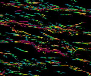
Figure 5 shows the scale energy in the  $r_1-r_3$ plane in the viscous sublayer and log-law layer. The green lines are obtained from a series of
  $(r_{1},r_{3})$ with
  $\min \{\langle \delta u^2 \rangle \}$ for every ring (
 $r_{1}^2+r_{3}^2=\textrm {const.}$). As indicated by the relation between the scale energy and the two-point correlation, at the scale
  $r={(r_1^2+r_3^2)^{1/2}}$, the angle
  $\tan ^{-1}\{r_1/r_3\}$ with
  $\min \{\langle \delta u^2 \rangle \}$ represents the direction of the vortices. Then, the green lines are fitted through the nonlinear least squares method with
  $R^2>0.8$ to obtain the inclination angles
  $\theta$, which are shown by the green labels and blue lines. As shown in figures 5(a) and 5(b), in the viscous sublayer of ST30, small-scale structures (
 $r_1^+\lessapprox 500$) form a strong angle with the rotation axis (up to
  $16^{\circ }$), while large-scale structures have a much smaller angle (approximately
  $3^{\circ }$). The threshold between small- and large-scale structures is determined to obtain reliable fitting results (
 $R^2>0.8$). The comparison between the results in the viscous sublayer (figure 5b) and those in the log-law layer (figure 5c) shows that energetic motions are distributed over a wider scale range in the log-law layer. In addition, as shown by the green lines, even if the small-scale inclination angles in the two layers are close to each other, the thresholds defined by strong inclination angles are far smaller in the log-law layer. The thresholds are
  $r_1^+=235.6$ and
  $r_3^+=49.0$ in the viscous sublayer, and they are
  $r_1^+=141.4$ and
  $r_3^+=23.6$ in the log-law layer. The three components of
  $\langle \delta u^2 \rangle$ have similar small-scale distributions, but
  $\langle \delta u_2^2 \rangle$ has a smaller amplitude and no obvious large-scale motion, which is not shown here for simplification.

Figure 5. Scale energy  $\langle \delta u^2 \rangle ^+/2$ of ST30 on the
  $r_1^+-r_3^+$ plane. (a) Large-scale distribution in the viscous sublayer (
 $x_2^+=3.5$). (b) Small-scale distribution in the viscous sublayer. (c) Small-scale distribution in the log-law layer (
 $x_2^+=80.0$). The green lines represent the directions of the coherent structures at certain scales. The green labels and blue lines are the fitting results of the green lines.
The details about the inclination angles  $\theta$ are displayed in figure 6. From the wall to the channel centre, the inclination angle
  $\theta$ decreases in most cases. At the channel centre,
  $\theta$ is exactly zero due to the antisymmetry in the wall-normal direction. Moreover, consistent with the observation of Dai et al. (Reference Dai, Huang and Xu2019), as
  $Ro_\tau$ becomes larger, the inclination angle of large-scale structures initially increases until
  $Ro_\tau =7$ and then decreases thereafter. When
  $Ro_\tau =60$, there is no apparent inclination angle (
 $\theta \approx 1^\circ$). Furthermore, as the rotation becomes stronger, the discrepancy between small-scale and large-scale structures is intensified. The most remarkable discrepancy occurs in the viscous sublayer of ST60S:
  $\theta$ at small scales is
  $19.0^\circ$, while at large scales is
  $1.1^\circ$. The multiscale inclined structures will be further quantitatively discussed in § 4.

Figure 6. Inclination angles  $\theta$ obtained based on the scale energy in different layers. (a) Small-scale inclination angles. (b) Large-scale inclination angles.
3.2. Basic results of the GKE
The budget equation of the scale energy, i.e. the GKE, can be written as (Marati et al. Reference Marati, Casciola and Piva2004)
 \begin{align} &\underbrace{\vphantom{\left\langle \frac{\partial^2}{\partial X_2^2}\right\rangle} -\frac{1}{2}\frac{\partial }{\partial r_j} \langle \delta u^2 \delta u_j \rangle }_{T^{SS}} \underbrace{\vphantom{\left\langle \frac{\partial^2}{\partial X_2^2}\right\rangle} -\frac{1}{2}\frac{\partial }{\partial X_2}\langle \delta u^2 u_2^\ast \rangle}_{T^{SP}} \underbrace{\vphantom{\left\langle \frac{\partial^2}{\partial X_2^2}\right\rangle} -\langle \delta u_1 \delta u_2 \rangle \left\langle\frac{\partial U_1}{\partial x_2} \right\rangle^\ast{-}\langle \delta u_2 \delta u_3 \rangle \left\langle\frac{\partial U_3 }{\partial x_2} \right\rangle^\ast }_{\varPi^{S}}\nonumber\\ &\quad \underbrace{\vphantom{\left\langle \frac{\partial^2}{\partial X_2^2}\right\rangle} -\frac{1}{\rho}\frac{\partial }{\partial X_2}\langle \delta u_2\delta p_R \rangle}_{P^S_R} \underbrace{\vphantom{\left\langle \frac{\partial^2}{\partial X_2^2}\right\rangle} -\frac{1}{\rho}\frac{\partial }{\partial X_2}\langle \delta u_2\delta p_T \rangle}_{P^S_T} +\underbrace{\vphantom{\left\langle \frac{\partial^2}{\partial X_2^2}\right\rangle} \nu \frac{\partial^2 }{\partial r_j \partial r_j} \langle \delta u^2 \rangle}_{D^{SS}}\nonumber\\ &\quad +\underbrace{\vphantom{\left\langle \frac{\partial^2}{\partial X_2^2}\right\rangle} \frac{\nu}{4}\frac{\partial^2}{\partial X_2^2} \langle \delta u^2 \rangle}_{D^{SP}} \underbrace{\vphantom{\left\langle \frac{\partial^2}{\partial X_2^2}\right\rangle} -2 \langle \epsilon^\ast \rangle}_{{-}E^{S}}=0, \end{align}
where  $T^{SS}$ and
  $T^{SP}$ are the turbulent convections in scale and spatial space,
  $\varPi ^{S}$ is the production,
  $P^{S}_R$ and
  $P^{S}_T$ are the pressure transfers induced by rotation and convection,
  $D^{SS}$ and
  $D^{SP}$ are the interscale and spatial viscous diffusions,
  $E^S$ is the pseudo-dissipation,
  $\epsilon =\nu ({\partial u_i}/{\partial x_j})({\partial u_i}/{\partial x_j})$ and ‘
 $\ast$’ represents the average of the values at
  $\boldsymbol {x}$ and
  $\boldsymbol {x}'$.
For multiscale analyses, there are three main methods: spectral, two-point correlation and second-order structure function approaches. The spectral method is the Fourier transform of two-point correlations (Pope Reference Pope2000). The relations between the second-order structure functions and the two-point correlations could be of interest and are given in Appendix A. These relations also have important practical applications in numerical postprocessing with high precision. In  $\boldsymbol {r}$ space, since the field is not periodic or infinitely smooth, the partial derivatives
  $\partial /\partial r_1$ and
  $\partial /\partial r_3$ cannot be directly calculated by the Fourier transform. To overcome this difficulty, utilizing the relations between the second-order structure functions and the two-point correlations, the partial derivatives
  $\partial /\partial r_i$ can be expanded in terms of
  $\partial /\partial x_i$ and
  $\partial /\partial x_i'$. With the relations in Appendix A, all terms of the GKE can be written as two-point correlations. Then, the derivatives can be solved by the Fourier transform. In addition, when
  $r\rightarrow \infty$, the scale energy will be reduced to four times the TKE, and the GKE will be reduced to the TKE budget equation (Marati et al. Reference Marati, Casciola and Piva2004; Hu et al. Reference Hu, Li and Yu2022). As shown in figure 4(c), the scale energy in the spanwise direction is almost unaffected by rotation. Therefore, the results with
  $r_{2}=r_{3}=0$ are the focus of this section.
The results for ST00 and ST30 in the viscous sublayer are given in figures 7(a) and 7(b), respectively. The main results are shown in logarithmic coordinates, and a breakpoint is inserted at the beginning of the abscissa to display the results at  $r_1^+=0$.

Figure 7. Budget balance of the GKE in the viscous sublayer ( $x_2^+=3.5$). The grey dashed lines represent the breakpoint to show the origin
  $r_1^+=0$ in logarithmic coordinates. Results are shown for (a) ST00 and (b) ST30.
In terms of the reliability of postprocessing, the sum of all terms is almost zero. In addition, when  $r_1^+=0$, the viscous diffusion
  $D^{SS}$ and the pseudo-dissipation
  $E^{S}$ balance each other, while other terms are exactly zero. Specifically, as deduced by the relation (A7), when
  $r_1^+=0$,
  $D^{SS}$ and
  $E^{S}$ are two times the pseudo-dissipation
  $E$ in the TKE budget equation,
 \begin{align} D^{SS}(r_1=0,x_2)=E^{S}(r_1=0,x_2)= 2\nu\left\langle \frac{\partial u_i}{\partial x_{j}} \frac{\partial u_i}{\partial x_{j}} \right\rangle=2E(x_2), \end{align}
which is verified in figure 7. These observations verify our postprocessing approach that expands the GKE in terms of the two-point correlations in Appendix A.
As shown in figure 7(a), in the viscous sublayer of ST00, except for  $-E^S<0$ and
  $P_R\approx 0$, all terms are positive. The scale energy is transferred toward small scales or toward the wall by these positive terms and then dissipated by
  $E^S$. Specifically, there are four main effects in the viscous sublayer: the production
  $\varPi ^{S}$, the spatial and interscale viscous transfers (
 $D^{SP}$ and
  $D^{SS}$), and the pseudo-dissipation
  $E^S$. However, as shown by the TKE budget balance in figure 3, closer to the wall,
  $\varPi ^S$ is negligible compared with the viscous effects. Among the three viscous effects,
  $D^{SP}$ is less important, which means that the dynamics in the viscous sublayer is spatially local (Marati et al. Reference Marati, Casciola and Piva2004). In addition,
  $D^{SS}$ and
  $D^{SP}$ become the same when
  $r_1\rightarrow \infty$.
The results for ST30 are shown in figure 7(b). In ST30,  $\varPi ^S$ is larger than that in ST00. The combination of the GKE results in figure 7 and the TKE budget balance in figure 3 suggests that
  $\varPi ^S$ is distributed closer to the wall in ST30 than in ST00. The rotation-induced pressure transfer
  $P_R^S$ is positive and is an additional direct transfer toward the wall. Furthermore, except for
  $\varPi ^S$,
  $P_R^S$ and
  $E^S$, the terms are suppressed by rotation. This means that rotation strengthens the near-wall turbulence mainly by directly producing more energy (
 $\varPi ^S$) and by the spatial pressure transfer induced by rotation (
 $P_R^S$), while other transfers between the viscous layer and the buffer layer are reduced. In fact, as shown by the TKE budget balance in figure 3, in the lower viscous layer, rotation makes the viscous effects stronger. This is mainly related to the stronger spanwise TKE
  $\langle u_3u_3 \rangle$. For the scale distribution,
  $\varPi ^S$ is distributed among
  $r_1^+\in (0, 10^3)$ in ST00 and among
  $r_1^+\in (0, 10^2)$ in ST30. This is consistent with the scale energy in figure 4(a), while the discrepancy is more apparent for
  $\varPi ^S$. In other words, rotation shortens the streamwise structures in the viscous sublayer. The results are non-trivial because rotation generally induces long streamwise coherent structures, such as TGL vortices (Yang & Wang Reference Yang and Wang2018). The shorter streamwise structures are partly caused by corresponding larger inclination angles at small scales. As shown in figure 5(a), the inclination angle of small-scale structures in the viscous sublayer is
  $16^\circ$. If only the slice with
  $r_3^+=0$ is considered, then the streamwise scales become smaller.
In the buffer layer, as shown in figure 8(a), at large scales ( $r_1^+>10^3$), only
  $\varPi ^S$ is positive. Therefore, energy is produced by
  $\varPi ^S$. Then, energy is transferred to other scales by interscale transfers (
 $D^{SS}$ and
  $T^{SS}$) and to other locations (up to the bulk of the flow and down to the viscous sublayer) by
  $T^{SP}$ and
  $D^{SP}$ or dissipated by
  $E^S$. In addition, the interscale transfers
  $T^{SS}$ and
  $D^{SS}$ are both positive at small scales but negative at large scales. On the one hand, energy is forward cascaded to small scales. On the other hand, if integrated in the
  $r_1$ direction, the fluxes are negative at large scales, which represents an inverse cascade. The dual cascades to smaller and larger scales are the reflection of breakdown, regeneration and coalescence of streamwise vortices (Hamilton, Kim & Waleffe Reference Hamilton, Kim and Waleffe1995). Furthermore, the interscale transfers are important at small scales, while the spatial effects are mainly valid at large scales. The pressure transfers (
 $P_R^S$ and
  $P_T^S$) are negligible and mainly redistribute the scale energy between different components (Yang & Wang Reference Yang and Wang2018).

Figure 8. Budget balance of the GKE in the buffer layer ( $x_2^+=10.5$). The grey dashed lines represent the breakpoint to show the origin
  $r_1^+=0$ in logarithmic coordinates. Results are shown for (a) ST00 and (b) ST30.
The comparison of figures 8(a) and 8(b) shows that when strong rotation is introduced, at large scales,  $\varPi ^S$ is not affected, while
  $E^S$ in the buffer layer is strongly reduced. At small scales (
 $r_1^+\lessapprox 10^2$), since
  $E^S$ balances with the interscale transfers (
 $T^{SS}$ and
  $D^{SS}$), the local interscale transfers are also reduced by rotation. At large scales (
 $r_1^+\gtrapprox 10^2$), the interscale and spatial turbulent convections (
 $T^{SS}$ and
  $T^{SP}$) are both strengthened by rotation. These observations imply that the forward cascades to small scales in the buffer layer are reduced by rotation, and instead, the scale energy is mainly spatially transported in the wall-normal direction or inversely cascaded. Additionally, as occurs in the viscous sublayer, the scale distribution of the production is also restricted by rotation in the buffer layer, indicating the presence of strongly inclined small-scale structures here.
In the log-law layer, as shown in figure 9(a), when there is no rotation,  $\varPi ^S$ is locally balanced with
  $E^S$ at large scales. The spatial and interscale transfers at large scales are negligible, and the log-law layer does not obtain or lose energy. In fact, energy is produced in the buffer layer and then transferred across the log-law layer toward the channel centre (Marati et al. Reference Marati, Casciola and Piva2004). Furthermore, the comparison of figure 8(a) and figure 9(a) shows that if normalized by
  $\varPi ^S$, the interscale transfers (
 $D^{SS}$ and
  $T^{SS}$) at small scales in the log-law layer are relatively more important than those in the buffer layer. The relatively weak spatial transfers and stronger interscale transfers mean that in the log-law layer the scale energy is locally cascaded to small-scale structures.

Figure 9. Budget balance of the GKE in the log-law layer ( $x_2^+=81.6$ for ST07R and
  $x_2^+=80.0$ for other cases). The grey dashed lines represent the breakpoint to show the origin
  $r_1^+=0$ in logarithmic coordinates. Results are shown for (a) ST00, (b) ST30, (c) ST07, (d) ST07R.
When rotation is introduced, as shown in figure 9(b), the local balance of  $\varPi ^S$ and
  $E^S$ is destroyed. Remarkable spatial energy transfers (
 $T^{SP}$ and
  $P^S_T$) are introduced, originating from the elongated large-scale streamwise vortices, according to the Reynolds stresses and their budget balance given by Yang & Wang (Reference Yang and Wang2018). Additionally, similar to the phenomena in the buffer layer, in the log-law layer the pseudo-dissipation (
 $E^{S}$) and the interscale transfers (
 $D^{SS}$ and
  $T^{SS}$) at small scales are also reduced by rotation. In fact, as shown in figure 4(b), in the log-law layer the scale energy at small scales is also reduced by rotation. In terms of the scale distribution, different from the results in the former two layers, in the log-law layer the scale distribution of all terms is extended to a much wider range by rotation. This means that rotation extends the streamwise structures in the log-law layer but shortens those in the viscous sublayer and the buffer layer, which could also be associated with the smaller inclination angle and narrower small-scale range in the log-law layer, as shown by the scale energy in figure 5(b,c).
Cases ST07 and ST07R are compared here to examine the effects of the Reynolds numbers. Figure 9(c,d) shows that the difference in the GKE results is mainly concentrated in the log-law layer, while the other layers are not shown in this paper because they are less affected by the Reynolds numbers. The comparison of figure 9(c,d) shows that at large scales, the spatial and interscale turbulent convections ( $T^{SP}$ and
  $T^{SS}$) are far smaller under larger Reynolds numbers. For these turbulent convections, smaller rotation numbers and larger Reynolds numbers have similar effects, as shown by the comparison of figure 9(a,c,d). In addition,
  $\varPi ^S$ and
  $E^S$ are larger with a higher Reynolds number, as the turbulence is strengthened. Strictly speaking, the layer
  $x_2^+\approx 80$ with
  $Re_\tau =180$ does not fully scale in viscous units and is located at the junction between the inner and outer layers. If larger Reynolds numbers are considered, then these results may be invariant with respect to the Reynolds number, similar to those in the viscous sublayer and the buffer layer.
In conclusion, rotation extracts more energy from the buffer layer to other layers. In the viscous sublayer the turbulence intensity is mainly strengthened by the movement of the production peak and the intensive spatial viscous diffusion. In the log-law layer the turbulence is mainly strengthened by the spatial turbulent convection, the inhibited forward cascades and the thus weaker pseudo-dissipation. In fact, in homogeneous rotating turbulence (Mininni et al. Reference Mininni, Alexakis and Pouquet2009), forward cascade inhibition has also been confirmed, attributed to the decay of non-resonant interactions. In streamwise-rotating channel turbulence the structures in the log-low layer are strongly elongated by rotation. In contrast, those structures under the buffer layer are shortened. This could be attributed to the strongly inclined structures near the wall, which will be investigated in § 4. Furthermore, increasing Reynolds numbers result in weaker spatial turbulent convection and stronger interscale transfers, which is opposite to the rotation effects. This is associated with the relative importance between inertial motions and the rotation effects. Similarly, in homogeneous rotating turbulence, under rapid rotation ( $\varOmega \rightarrow \infty$), the nonlinear turbulent convection is negligible (Davidson Reference Davidson2013).
4. Inclined structures and sustaining mechanisms
In § 3.1 it has been found that the inclination angles of large- and small-scale structures are completely different, and the difference is more remarkable as rotation becomes stronger. In this section we use the angle based on the velocity vector and the filtering approach to identify these inclined structures more quantitatively. Then, based on the related budget balance of the Reynolds stresses and AGKE for the second-order structure functions, we identify the key sustaining mechanisms for small-scale inclined structures, with further physical explanations provided through the hairpin vortex model. Finally, the scale discrepancy will also be discussed in detail.
4.1. Identification of the inclined structures
To confirm these observations about the inclined structures, figure 10 shows the vortex structures under the log-law layer ( $x_2^+<90$) for the cases (a) ST00, (b) ST07 and (c) ST30. The structures are coloured by the distance from the wall and are shown with
  $Q>500$, where
  $Q=[2|\boldsymbol {\nabla } \times \boldsymbol {u}|^2-|\boldsymbol {\nabla } \boldsymbol {u} +(\boldsymbol {\nabla } \boldsymbol {u})^T|^2]/8$. The white solid lines in (b) and (c) are given for reference of the inclination angles. As shown, the structures of ST07 and ST30 have larger lateral sizes than those of ST00, in agreement with the observation in figure 4(c). Furthermore, in figure 10(a) the structures of ST00 are fully aligned with the streamwise direction in all layers, where no rotation is introduced. The structures of ST07 are shown in figure 10(b). The structures have a small inclination angle (
 $8.0^\circ$). Figure 10(c) gives the results for ST30. Most small-scale structures (
 ${\rm \Delta} x_1^+<500$) have an angle of
  $16.0^\circ$. However, the large-scale structures (
 ${\rm \Delta} x_1^+>2000$) display angles between
  $2.63^\circ$ and
  $16.0^\circ$. In what follows, these structures will be identified by a more quantitative method.

Figure 10. Flow structures under the log-law layer ( $x_2^+<90$) with
  $Q>500$ for the cases (a) ST00, (b) ST07, (c) ST30. The structure is coloured by
  $x_2^+$, with the colour bar on the right of panel (a). The white lines and labels are given for reference.
For channel turbulence, researchers (Kim & Moin Reference Kim and Moin1986; Jiménez Reference Jiménez2011) usually use the velocity direction to recognize sweeps and ejections. Therefore, the inclination angle can be defined by the velocity field as
 \begin{equation} \theta_u=\tan^{{-}1} \{u_3/u_1\} . \end{equation}
To illustrate the scale discrepancy, filtering methods are used to isolate the large- and small-scale results. The large- and small-scale angles are defined as
 \begin{equation} \theta_{u,L}(\boldsymbol{x})=\tan^{{-}1} \left\{\frac{\displaystyle \int G_L(\boldsymbol{r}) u_{3}(\boldsymbol{x}-\boldsymbol{r})\mathrm{d} \boldsymbol{r}}{\displaystyle \int G_L(\boldsymbol{r}) u_{1}(\boldsymbol{x}-\boldsymbol{r})\mathrm{d} \boldsymbol{r}} \right\}, \quad \theta_{u,S}(\boldsymbol{x})=\tan^{{-}1} \left\{\frac{\displaystyle \int G_S(\boldsymbol{r}) u_{3}(\boldsymbol{x}-\boldsymbol{r})\mathrm{d} \boldsymbol{r}}{\displaystyle \int G_S(\boldsymbol{r}) u_{1}(\boldsymbol{x}-\boldsymbol{r})\mathrm{d} \boldsymbol{r}} \right\}, \end{equation}
where  $G_L$ and
  $G_S$ are corresponding filters. To avoid any artificial effects on the vortex direction, the same filter width is used in the streamwise and spanwise directions. Three filters and three filter widths are considered in Appendix B. Although affected by filters, the small-scale results manifest the same tendency. The large-scale results exhibit a similar distribution to the non-filtered results but are sensitive to the filter width. In our study,
  $\varDelta _L\in [0.1{\rm \pi},0.4{\rm \pi} ]$ and is comparable to the width of two-layer TGL vortices (
 $0.16{\rm \pi}$). The TGL vortices have been studied by many researchers (Yang & Wang Reference Yang and Wang2018) and are not the subject of this paper. In the following analysis, only the small-scale results with the Gaussian filters ((B1)) of
  $\varDelta _S=0.025{\rm \pi}$ are presented.
The results are given in figure 11. As shown in figure 11(a), in the low log-law layer ( $x_2^+\approx 40$ and
  $x_2\approx \pm 0.75$), as rotation becomes stronger, the average large-scale inclination angle
  $\langle \theta _{u,L} \rangle$ decreases. However, in the vicinity of the wall and around the channel centre,
  $\langle \theta _{u,L} \rangle$ is roughly unchanged for different cases. This should be attributed to the local distribution of a large-scale streamwise vortex, which is the limit of the inclination angle based on the velocity vector. However, the average small-scale angle
  $\langle \theta _{u,S} \rangle$ has completely different distributions, as shown in figure 11(b). As rotation intensifies,
  $\langle \theta _{u,S} \rangle$ near the wall (
 $x_2^+\approx 18$ and
  $x_2\approx \pm 0.1$) monotonically increases. In higher layers the
  $\langle \theta _{u,S} \rangle$ of ST60S is slightly smaller than that of ST30. Generally, this is consistent with the results shown in figure 6. There are also small differences, such as the specific values of angles, which can be attributed to their different definitions. Moreover, as
  $Re_\tau$ increases,
  $\langle \theta _{u,S} \rangle$ generally decreases. There could be two reasons. First, ST07R has a wider scale range, and the smallest scale is not affected by rotation, which is supported by the scale energy not shown. The second reason is the thinner boundary layer in ST07R. There is no inclination angle in homogeneous rotating turbulence. Roughly speaking, the inclined structures originate from the coupling effects of boundary layers and rotation. Case ST07R has a thinner boundary layer than ST07 and, thus, has a weaker inclination angle. This deduction can be verified by the fact that in figure 11 the
  $\langle \theta _{u,S} \rangle$ of ST07 and that of ST07R are almost the same under the viscous sublayer but are completely different away from the wall. Figure 12 shows the probability density function (PDF) of the small-scale inclination angle
  $\theta _{u,S}$ in (a) the buffer layer and (b) the low log-law layer. As rotation intensifies, the peaks of the PDF move toward a positive value. Furthermore, in the low log-law layer, the peaks have weaker amplitudes than those in the buffer layer, indicating an isotropic tendency away from the wall.

Figure 11. Comparison of the average inclination angles of different scales. (a) Average inclination angle  $\langle \theta _u \rangle$. (b) Average inclination angle at small scales
  $\langle \theta _{u,S} \rangle$.

Figure 12. Comparison of the PDF of the small-scale inclination angle  $\theta _{u,S}$ in (a) the buffer layer (
 $x_2^+=10.3$ for ST07R and
  $x_2^+=10.5$ for other cases) and (b) the low log-law layer (
 $x_2^+=46.6$ for all cases).
4.2. Sustaining mechanisms of the inclined structures
After the identification of the inclined structures, the focus is on the sustaining mechanisms of these structures. Since the distribution of  $\langle u_1u_3 \rangle$ is similar to that of
  $\langle \theta _u \rangle$, for simplification, the phenomena are analysed based on the budget balance of
  $\langle u_1u_3 \rangle$ and the AGKE of
  $\langle \delta u_1\delta u_3 \rangle$. For an overview of the mechanisms, the Reynolds stress budget equation is studied first and is written as
 \begin{align} &
\underbrace{\vphantom{\left\langle
\frac{\partial^2}{\partial X_2^2}\right\rangle} - \langle
u_2 u_j \rangle \frac{\mathrm{d} \langle U_i \rangle
}{\mathrm{d} x_2} - \langle u_2 u_i \rangle
\frac{\mathrm{d} \langle U_j \rangle }{\mathrm{d}
x_2}}_{\varPi_{ij}} +\underbrace{\vphantom{\left\langle
\frac{\partial^2}{\partial X_2^2}\right\rangle}2\varOmega
\langle \epsilon_{1im}u_ju_m+\epsilon_{1jm}u_iu_m \rangle
}_{{\mathsf{C}}_{ij}} \underbrace{\vphantom{\left\langle
\frac{\partial^2}{\partial
X_2^2}\right\rangle}-\frac{\mathrm{d} }{\mathrm{d}
x_2}\langle u_iu_ju_2 \rangle }_{{\mathsf{T}}_{ij}}
\nonumber\\ &\quad \underbrace{\vphantom{\left\langle
\frac{\partial^2}{\partial
X_2^2}\right\rangle}-\frac{1}{\rho}\left\langle u_j
\frac{\partial p_R}{\partial x_i} + u_i \frac{\partial
p_R}{\partial x_j} \right\rangle }_{{\mathsf{P}}_{R,ij}}
\underbrace{\vphantom{\left\langle
\frac{\partial^2}{\partial
X_2^2}\right\rangle}-\frac{1}{\rho}\left\langle u_j
\frac{\partial p_T}{\partial x_i} + u_i \frac{\partial
p_T}{\partial x_j} \right\rangle }_{{\mathsf{P}}_{T,ij}}\nonumber\\
&\quad +\underbrace{\vphantom{\left\langle
\frac{\partial^2}{\partial
X_2^2}\right\rangle}\nu\frac{\mathrm{d}^2}{\mathrm{d}
x_2^2}\langle u_iu_j \rangle} _{{\mathsf{D}}_{ij}}
\underbrace{\vphantom{\left\langle
\frac{\partial^2}{\partial X_2^2}\right\rangle}-2\nu
\left\langle \frac{\partial u_i}{\partial
x_k}\frac{\partial u_j}{\partial x_k} \right\rangle
}_{{-}{\mathsf{E}}_{ij}} =0,
\end{align}
\begin{align} &
\underbrace{\vphantom{\left\langle
\frac{\partial^2}{\partial X_2^2}\right\rangle} - \langle
u_2 u_j \rangle \frac{\mathrm{d} \langle U_i \rangle
}{\mathrm{d} x_2} - \langle u_2 u_i \rangle
\frac{\mathrm{d} \langle U_j \rangle }{\mathrm{d}
x_2}}_{\varPi_{ij}} +\underbrace{\vphantom{\left\langle
\frac{\partial^2}{\partial X_2^2}\right\rangle}2\varOmega
\langle \epsilon_{1im}u_ju_m+\epsilon_{1jm}u_iu_m \rangle
}_{{\mathsf{C}}_{ij}} \underbrace{\vphantom{\left\langle
\frac{\partial^2}{\partial
X_2^2}\right\rangle}-\frac{\mathrm{d} }{\mathrm{d}
x_2}\langle u_iu_ju_2 \rangle }_{{\mathsf{T}}_{ij}}
\nonumber\\ &\quad \underbrace{\vphantom{\left\langle
\frac{\partial^2}{\partial
X_2^2}\right\rangle}-\frac{1}{\rho}\left\langle u_j
\frac{\partial p_R}{\partial x_i} + u_i \frac{\partial
p_R}{\partial x_j} \right\rangle }_{{\mathsf{P}}_{R,ij}}
\underbrace{\vphantom{\left\langle
\frac{\partial^2}{\partial
X_2^2}\right\rangle}-\frac{1}{\rho}\left\langle u_j
\frac{\partial p_T}{\partial x_i} + u_i \frac{\partial
p_T}{\partial x_j} \right\rangle }_{{\mathsf{P}}_{T,ij}}\nonumber\\
&\quad +\underbrace{\vphantom{\left\langle
\frac{\partial^2}{\partial
X_2^2}\right\rangle}\nu\frac{\mathrm{d}^2}{\mathrm{d}
x_2^2}\langle u_iu_j \rangle} _{{\mathsf{D}}_{ij}}
\underbrace{\vphantom{\left\langle
\frac{\partial^2}{\partial X_2^2}\right\rangle}-2\nu
\left\langle \frac{\partial u_i}{\partial
x_k}\frac{\partial u_j}{\partial x_k} \right\rangle
}_{{-}{\mathsf{E}}_{ij}} =0,
\end{align}
where  $\varPi _{ij}$ is the production,
  ${\mathsf{C}}_{ij}$ is the Coriolis term,
  ${\mathsf{T}}_{ij}$ is the turbulent convection,
  ${\mathsf{D}}_{ij}$ is the viscous diffusion,
  ${\mathsf{E}}_{ij}$ is the pseudo-dissipation, and
  ${\mathsf{P}}_{R,ij}$ and
  ${\mathsf{P}}_{T,ij}$ are the pressure–velocity correlation terms related to the rotation effects and turbulent convection, respectively. Since
  ${\mathsf{C}}_{ij}$ and
  ${\mathsf{P}}_{R,ij}$ are both induced by rotation and are strongly cancelled by each other, the two terms are summed to form a new term
  ${\mathsf{C}}_{ij,\textit{eff}}$ (Yang et al. Reference Yang, Deng, Wang and Shen2020a).
The budget balance for the Reynolds stresses ( $\langle u_1u_3 \rangle$ and
  $\langle u_2u_3 \rangle$) of ST30 is given in figure 13. The terms in figure 13 have opposite signs to those reported by Yang & Wang (Reference Yang and Wang2018) due to the different domain ranges evaluated. Specifically, this study examines the upper domain (
 $x_2\in [0,1]$), while Yang & Wang (Reference Yang and Wang2018) explored the lower domain (
 $x_2\in [-1,0]$). As shown in figure 13(a), the effective Coriolis term
  ${\mathsf{C}}_{13,{eff}}$ reduces the inclination angle. In contrast, there are two main sources for
  $\langle u_1 u_3 \rangle$, i.e. the convection-induced pressure–velocity correlation term
  ${\mathsf{P}}_{T,13}$ and the production
  $\varPi _{13}$.
  ${\mathsf{P}}_{T,ij}$ can be simplified as
 \begin{equation} {\mathsf{P}}_{T,ij}={-}\frac{1}{\rho}\left\langle u_i \frac{\partial p_T}{\partial x_j} + u_j \frac{\partial p_T}{\partial x_i} \right\rangle ={-}\frac{1}{\rho}\left\langle \frac{\partial u_ip_T}{\partial x_j}+\frac{\partial u_jp_T}{\partial x_i} \right\rangle +\frac{2}{\rho}\langle p_T {\mathsf{S}}_{ij}\rangle, \end{equation}
where the strain rate tensor  ${\mathsf{S}}_{ij}=(\partial u_i/\partial x_j+\partial u_j /\partial x_i)/2$. Here,
  ${\mathsf{P}}_{T,13}= {2}\langle p_T {\mathsf{S}}_{13} \rangle /{\rho }$ and could be related to the strain rate tensor. To confirm the effect of the strain, the principal directions of the strain rate tensors (
 $\langle \theta _{{\mathsf{S}}_{ij}} \rangle$ and
  $\langle \theta _{{\mathsf{S}}_{ij},S} \rangle$) are calculated by the eigenvector with
  $\max \{|\lambda _i|\}$, where
  $\lambda _i$ is the eigenvalue. The principal directions of the strain rate tensors are given in figure 14. As shown, the tendency of
  $\langle \theta _{{\mathsf{S}}_{ij},S} \rangle$ is similar to that of
  $\langle \theta _{u,S} \rangle$ in figure 11. On the one hand, the strain tries to induce these inclined structures via
  ${\mathsf{P}}_{T,13}$. On the other hand, the strain also affects the dissipation, which reduces the inclination angle. Another more important source is the production
  $\varPi _{13}$, which can be decomposed into two components (
 $\varPi _{13,1}$ and
  $\varPi _{13,2}$), i.e.,
 \begin{equation} \varPi_{13}= \underbrace{-\langle u_2u_3 \rangle \frac{\mathrm{d} \langle U_1 \rangle }{\mathrm{d} x_2}}_{\varPi_{13,1}} \underbrace{-\langle u_1u_2 \rangle \frac{\mathrm{d} \langle U_3 \rangle}{\mathrm{d} x_2}}_{\varPi_{13,2}}. \end{equation}
Figure 15 gives (a) the production and (b,c) its decomposition. The production  $\varPi _{13}$ is the main reason for the inclination angle. It is positive in the buffer layer but negative in higher layers. As rotation intensifies, the positive peak moves towards the wall and has a larger value. The decomposition in figure 15(b,c) shows that
  $\varPi _{13,1}$ is responsible for the positive peaks, especially for strongly rotating cases (ST30 and ST60S). Here,
  $\varPi _{13,1}$ originates from the Reynolds stress
  $\langle u_2u_3 \rangle$. As shown in figure 13(b), the effective Coriolis term
  ${\mathsf{C}}_{23,{eff}}$ is the only source for positive
  $\langle u_2u_3 \rangle$. In other words,
  ${\mathsf{C}}_{23,{eff}}$ induces positive
  $\langle u_2u_3 \rangle$, and then, under the strain induced by
  $\langle U_1 \rangle$,
  $\langle u_2u_3 \rangle$ further leads to these inclined structures. Notably, Yang et al. (Reference Yang, Deng, Wang and Shen2020a) found that
  $\langle u_2u_3 \rangle$ constrains itself from increasing infinitely. From
  $\varPi _{13,1}$, it can be inferred that with stronger rotation, the inclination angle also cannot infinitely increase, as confirmed by the
  $\langle \theta _{u,S} \rangle$ of ST30 and ST60S in figure 11.

Figure 13. Budget balance of  $\langle u_i u_j \rangle ^+$ for ST30: (a)
  $\langle u_1 u_3 \rangle ^+$, (b)
  $\langle u_2 u_3 \rangle ^+$.

Figure 14. Comparison of the average inclination angles given by the principal directions of the strain rate tensor. (a) Average inclination angle  $\langle \theta _{{\mathsf{S}}_{ij}} \rangle$. (b) Average inclination angle at small scales
  $\langle \theta _{{\mathsf{S}}_{ij},S} \rangle$.

Figure 15. Production decomposition for the budget balance of  $\langle u_1 u_3 \rangle ^+$. Results are shown for (a)
  $\varPi _{13}^+$,(b)
  $\varPi _{13,1}^+$, (c)
  $\varPi _{13,2}^+$.
To illustrate how these strongly inclined small-scale structures are sustained under rotation, a simple hairpin vortex model is proposed here. To be consistent with the previous analysis, the upper channel domain ( $x_2\in [0,1]$) is considered. It is in a left-handed coordinate system because a transform of
  $x_2\leftarrow 1-x_2$ is used when the upper domain is discussed. For a clearer illustration, the three main effects can be summarized as
 \begin{equation}
\left.\begin{array}{@{}c@{}} \displaystyle \varPi_{13,1}=
\left\langle u_3\left({-}u_2\dfrac{\mathrm{d}{} \langle U_1
\rangle }{\mathrm{d}{} x_2}\right) \right\rangle = \langle
u_3 F_{\varPi 1} \rangle \quad \textrm{for}\ \left\langle
u_3\dfrac{\partial u_1}{\partial t} \right\rangle,\\
\displaystyle {\mathsf{C}}_{23}\approx \langle u_3(2\varOmega u_3)
\rangle = \langle u_3 F_{C2} \rangle \quad \textrm{for}
\left\langle u_3\dfrac{\partial u_2}{\partial t}
\right\rangle,\\ \displaystyle {\mathsf{C}}_{13}= \langle
u_1({-}2\varOmega u_2) \rangle = \langle u_1 F_{C3} \rangle
\quad \textrm{for} \left\langle u_1\dfrac{\partial
u_3}{\partial t} \right\rangle,\\ \end{array}\right\}
\end{equation}
\begin{equation}
\left.\begin{array}{@{}c@{}} \displaystyle \varPi_{13,1}=
\left\langle u_3\left({-}u_2\dfrac{\mathrm{d}{} \langle U_1
\rangle }{\mathrm{d}{} x_2}\right) \right\rangle = \langle
u_3 F_{\varPi 1} \rangle \quad \textrm{for}\ \left\langle
u_3\dfrac{\partial u_1}{\partial t} \right\rangle,\\
\displaystyle {\mathsf{C}}_{23}\approx \langle u_3(2\varOmega u_3)
\rangle = \langle u_3 F_{C2} \rangle \quad \textrm{for}
\left\langle u_3\dfrac{\partial u_2}{\partial t}
\right\rangle,\\ \displaystyle {\mathsf{C}}_{13}= \langle
u_1({-}2\varOmega u_2) \rangle = \langle u_1 F_{C3} \rangle
\quad \textrm{for} \left\langle u_1\dfrac{\partial
u_3}{\partial t} \right\rangle,\\ \end{array}\right\}
\end{equation}
where  $-2\varOmega \langle u_2u_2 \rangle$ in
  ${\mathsf{C}}_{23}$ is negligible compared with
  $2\varOmega \langle u_3u_3 \rangle$. In (4.6),
  $F_{\varPi 1}, F_{C2},$ and
  $F_{C3}$ are the corresponding forces of the three key terms
  $\varPi _{13,1}, {\mathsf{C}}_{23}$ and
  ${\mathsf{C}}_{13}$, respectively. The forces directly affect the momentum and, thus, the Reynolds stresses
  $\langle u_1u_3 \rangle$ and
  $\langle u_2u_3 \rangle$. The analysis of the three forces on a vortex could give some intuitions about the mechanisms shown by the Reynolds stress budget balance. In figure 16 two events of a hairpin vortex are considered: (a) ejections with
  $\{u_1<0,u_2<0,u_3<0\}$ and (b) sweeps with
  $\{u_1>0,u_2>0,u_3>0\}$. As shown by the black arrows, fluid ejects mainly in the inboard of the vortex and sweeps mainly in the outboard region (Adrian Reference Adrian2007). The assumption of
  $u_1$ and
  $u_2$ is based on the ejection and sweep models of the hairpin vortex (Jiménez Reference Jiménez2011). The models are still effective in streamwise-rotating channel turbulence because the distribution of
  $\langle u_1u_2 \rangle$ is almost unaffected by the streamwise rotation (Yang & Wang Reference Yang and Wang2018), and hairpin vortexes are also observed in ST07 in figure 10. Notably, contrary to the classical hairpin vortex model, since the upper domain is considered here,
  $u_2<0$ for the ejections and
  $u_2>0$ for the sweeps. In addition, due to
  $\langle \theta _{u,S} \rangle$ in figure 11,
  $u_3$ is selected to have the same sign as
  $u_1$. Based on the hairpin vortex model in figure 16, the effects of the forces on the ejection and sweep are illustrated separately.
(i) As shown in figure 16(a), in the ejection, the Coriolis force
 $F_{C3}$ tries to induce a positive spanwise velocity $u_3$, which is opposite to the assumption $u_3<0$. Since $u_1<0$, $u_1F_{C3}<0$. This is consistent with the negative term ${\mathsf{C}}_{13,{eff}}$ in figure 13(a) and is the direct mechanism of ${\mathsf{C}}_{13,{eff}}$ reducing the positive inclination angle. In contrast, since $u_3<0$, $F_{C2}$ tries to induce negative $u_2$, consistent with the ejection assumption of $u_2<0$. Then, as $u_2<0$, $F_{\varPi 1}$ related to $\varPi _{13,1}$ tries to induce negative $u_1$, and thus, $u_3F_{\varPi 1}>0$. The effects of the forces $F_{C2}$ and $F_{\varPi 1}$ are consistent with the budget balance of $\langle u_2u_3 \rangle$ and $\langle u_1u_3 \rangle$. This mechanism is responsible for the small-scale inclined structures near the wall. Here $F_{C2}$ strengthens the wall-normal velocity and $F_{\varPi 1}$, which further induces the inclination structures.
(ii) As shown in figure 16(b), in the sweep,
$F_{C3}$ leads to a negative spanwise velocity $u_3$ and $u_1F_{C3}<0$, which reduces the positive inclination angle; $F_{C2}$ tries to induce positive $u_2$; $F_{\varPi 1}$ intensifies the positive $u_1$, and thus, $u_3F_{\varPi 1}>0$. The effects of the three forces are also consistent with the budget balance of $\langle u_2u_3 \rangle$ and $\langle u_1u_3 \rangle$.


Figure 16. Three forces in the (a) ejection and (b) sweep of a hairpin vortex. The upper half-domain is given to be consistent with the above analysis, and thus, the left-handed system is used. The black arrows give the main region of ejections and sweeps, and the dark blue arrows show the force directions.
Through this hairpin vortex model, the physical processes hidden under the Reynolds stress budget balance are clearly shown. In conclusion, there are two main mechanisms. First,  ${\mathsf{C}}_{13}$ related to
  $F_{C3}$ directly reduces the inclination angle. In contrast,
  ${\mathsf{C}}_{23}$ related to
  $F_{C2}$ indirectly induces a positive
  $\langle u_2u_3 \rangle$, which then results in inclination structures under the mean shear stress induced by
  $\varPi _{13,1}$.
To further confirm the findings, the scale decompositions are considered using the AGKE, which was deduced by Gatti et al. (Reference Gatti, Chiarini, Cimarelli and Quadrio2020) for inhomogeneous turbulence. In channel turbulence with streamwise rotation, the AGKE is written as
 \begin{align} 0&=
\underbrace{\vphantom{\left\langle
\frac{\partial^2}{\partial X_2^2}\right\rangle} - \langle
\delta u_j \delta u_2 \rangle \left\langle \frac{\partial
U_i}{\partial X_2} \right\rangle^\ast{-} \langle \delta u_i
\delta u_2 \rangle \left\langle \frac{\partial
U_j}{\partial X_2} \right\rangle ^\ast }
_{\varPi^{S}_{ij}}
+\underbrace{\vphantom{\left\langle
\frac{\partial^2}{\partial X_2^2}\right\rangle} 2\varOmega
(\varepsilon_{1im}\langle \delta u_j\delta u_m \rangle
+\varepsilon_{1jm}\langle \delta u_i\delta u_m \rangle )
}_{{\mathsf{C}}^{S}_{ij}}\nonumber\\ &\quad
\underbrace{\vphantom{\left\langle
\frac{\partial^2}{\partial X_2^2}\right\rangle}
-\frac{\partial }{\partial X_2} \langle \delta u_i \delta
u_j u_2^\ast\rangle }_{{\mathsf{T}}^{SP}_{ij}}
\underbrace{\vphantom{\left\langle
\frac{\partial^2}{\partial X_2^2}\right\rangle}
-\frac{\partial }{\partial r_k} \langle \delta u_i\delta
u_j \delta u_k \rangle }_{{\mathsf{T}}^{SS}_{ij}}
\underbrace{\vphantom{\left\langle
\frac{\partial^2}{\partial X_2^2}\right\rangle}
-\frac{1}{\rho}\left\langle \delta u_j\frac{\partial \delta
p_R}{\partial X_i} +\delta u_i\frac{\partial \delta
p_R}{\partial X_j} \right\rangle }_{{\mathsf{P}}^S_{R,ij}}\nonumber\\
&\quad \underbrace{\vphantom{\left\langle
\frac{\partial^2}{\partial X_2^2}\right\rangle}
-\frac{1}{\rho}\left\langle \delta u_j\frac{\partial \delta
p_T}{\partial X_i} +\delta u_i\frac{\partial \delta
p_T}{\partial X_j} \right\rangle }_{{\mathsf{P}}^S_{T,ij}}
+\underbrace{\vphantom{\left\langle
\frac{\partial^2}{\partial X_2^2}\right\rangle}
\frac{\nu}{2}\frac{\partial^2}{\partial X_2^2} \langle
\delta u_i\delta u_j \rangle }_{{\mathsf{D}}^{SP}_{ij}}
+\underbrace{\vphantom{\left\langle
\frac{\partial^2}{\partial X_2^2}\right\rangle} 2\nu
\frac{\partial^2}{\partial r_k\partial r_k}\langle \delta
u_i\delta u_j \rangle }_{{\mathsf{D}}^{SS}_{ij}}
\underbrace{\vphantom{\left\langle
\frac{\partial^2}{\partial X_2^2}\right\rangle} -4 \langle
\epsilon_{ij} \rangle ^\ast}_{{-}{\mathsf{E}}^S_{ij}},
\end{align}
\begin{align} 0&=
\underbrace{\vphantom{\left\langle
\frac{\partial^2}{\partial X_2^2}\right\rangle} - \langle
\delta u_j \delta u_2 \rangle \left\langle \frac{\partial
U_i}{\partial X_2} \right\rangle^\ast{-} \langle \delta u_i
\delta u_2 \rangle \left\langle \frac{\partial
U_j}{\partial X_2} \right\rangle ^\ast }
_{\varPi^{S}_{ij}}
+\underbrace{\vphantom{\left\langle
\frac{\partial^2}{\partial X_2^2}\right\rangle} 2\varOmega
(\varepsilon_{1im}\langle \delta u_j\delta u_m \rangle
+\varepsilon_{1jm}\langle \delta u_i\delta u_m \rangle )
}_{{\mathsf{C}}^{S}_{ij}}\nonumber\\ &\quad
\underbrace{\vphantom{\left\langle
\frac{\partial^2}{\partial X_2^2}\right\rangle}
-\frac{\partial }{\partial X_2} \langle \delta u_i \delta
u_j u_2^\ast\rangle }_{{\mathsf{T}}^{SP}_{ij}}
\underbrace{\vphantom{\left\langle
\frac{\partial^2}{\partial X_2^2}\right\rangle}
-\frac{\partial }{\partial r_k} \langle \delta u_i\delta
u_j \delta u_k \rangle }_{{\mathsf{T}}^{SS}_{ij}}
\underbrace{\vphantom{\left\langle
\frac{\partial^2}{\partial X_2^2}\right\rangle}
-\frac{1}{\rho}\left\langle \delta u_j\frac{\partial \delta
p_R}{\partial X_i} +\delta u_i\frac{\partial \delta
p_R}{\partial X_j} \right\rangle }_{{\mathsf{P}}^S_{R,ij}}\nonumber\\
&\quad \underbrace{\vphantom{\left\langle
\frac{\partial^2}{\partial X_2^2}\right\rangle}
-\frac{1}{\rho}\left\langle \delta u_j\frac{\partial \delta
p_T}{\partial X_i} +\delta u_i\frac{\partial \delta
p_T}{\partial X_j} \right\rangle }_{{\mathsf{P}}^S_{T,ij}}
+\underbrace{\vphantom{\left\langle
\frac{\partial^2}{\partial X_2^2}\right\rangle}
\frac{\nu}{2}\frac{\partial^2}{\partial X_2^2} \langle
\delta u_i\delta u_j \rangle }_{{\mathsf{D}}^{SP}_{ij}}
+\underbrace{\vphantom{\left\langle
\frac{\partial^2}{\partial X_2^2}\right\rangle} 2\nu
\frac{\partial^2}{\partial r_k\partial r_k}\langle \delta
u_i\delta u_j \rangle }_{{\mathsf{D}}^{SS}_{ij}}
\underbrace{\vphantom{\left\langle
\frac{\partial^2}{\partial X_2^2}\right\rangle} -4 \langle
\epsilon_{ij} \rangle ^\ast}_{{-}{\mathsf{E}}^S_{ij}},
\end{align}
where  ${\mathsf{T}}^{SS}_{ij}$ and
  ${\mathsf{T}}^{SP}_{ij}$ are the turbulent convections in scale and spatial space,
  $\varPi ^{S}_{ij}$ is the production,
  ${\mathsf{P}}^{S}_{ij,R}$ and
  ${\mathsf{P}}^{S}_{ij,T}$ are the pressure–velocity correlation terms induced by rotation and convection,
  ${\mathsf{D}}^{SS}_{ij}$ and
  ${\mathsf{D}}^{SP}_{ij}$ are the interscale and spatial viscous diffusion,
  ${\mathsf{E}}^{S}_{ij}$ is the pseudo-dissipation and
  $\epsilon _{ij}=\nu ({\partial u_i}/{\partial x_k})({\partial u_j}/{\partial x_k})$. Figure 17 shows the AGKE of
  $\langle \delta u_1 \delta u_3 \rangle$ for ST30 in the buffer layer (
 $x_2^+=10.5$). The main conclusion is consistent with that obtained based on the budget balance of
  $\langle u_1u_3 \rangle$. Therefore, it is reliable to use the budget balance of
  $\langle u_1u_3 \rangle$ to study the mechanisms for small-scale inclined structures. Furthermore, at small scales, there are still positive interscale turbulent convection
  ${\mathsf{T}}_{13}^{SS}$ and interscale viscous diffusion
  ${\mathsf{D}}_{13}^{SS}$, similar to the GKE results in figure 8. These strongly inclined structures are produced around
  $r_1^+\approx 100$ and then induce inclined structures at smaller scales via forward cascades.

Figure 17. The AGKE of  $\langle \delta u_1 \delta u_3 \rangle ^+$ for ST30 in the buffer layer (
 $x_2^+=10.5$).
Finally, the mechanisms underlying the discrepancy between small- and large-scale inclination angles observed based on  $\langle \theta _u \rangle$ and
  $\langle \theta _{u,S} \rangle$ are investigated. As shown in figure 11, in the low log-law layer (
 $x_2^+=46.6$), as
  $Ro_\tau$ increases from
  $0$ to
  $30$, the structures of overall scale have weaker inclination angles, but small-scale structures have stronger angles. According to the production decomposition in figure 15, the decaying angles for large-scale structures could be mainly attributed to the negative
  $\varPi _{13,2}$ in the log-law layer. According to the profile in figure 2 and the Reynolds stresses given by Yang & Wang (Reference Yang and Wang2018), in the boundary layer,
  $\langle u_1u_2 \rangle$ does not change its sign, while the behaviour is the opposite for
  $\partial \langle U_3 \rangle /\partial x_2$. Therefore, the mean spanwise velocity gradients could be responsible for the decaying angles of large-scale structures with increasing rotation rates. To further confirm the deduction, the production in the AGKE is also decomposed as follows:
 \begin{equation}
\varPi_{13}^{S}=\underbrace{- \langle \delta u_3 \delta u_2
\rangle \left\langle \frac{\partial U_1}{\partial X_2}
\right\rangle^\ast}_{\varPi_{13,1}^S} \underbrace{- \langle
\delta u_1 \delta u_2 \rangle \left\langle \frac{\partial
U_3}{\partial X_2} \right\rangle^\ast }_{\varPi_{13,2}^S}.
\end{equation}
\begin{equation}
\varPi_{13}^{S}=\underbrace{- \langle \delta u_3 \delta u_2
\rangle \left\langle \frac{\partial U_1}{\partial X_2}
\right\rangle^\ast}_{\varPi_{13,1}^S} \underbrace{- \langle
\delta u_1 \delta u_2 \rangle \left\langle \frac{\partial
U_3}{\partial X_2} \right\rangle^\ast }_{\varPi_{13,2}^S}.
\end{equation}
Figure 18 shows the decomposition for ST30 at  $x_2^+=46.6$, where panel (a) gives the overall production
  $\varPi _{13}^{S+}$ and panels (b,c) give the decomposition. As shown in figure 18(a), for ST30 and ST60S with strong scale discrepancies,
  $\varPi _{13}^{S}$ is positive at small scales but negative at large scales. For ST07 with no obvious discrepancy, the production is completely negative. As shown by the decomposition in figure 18(b,c),
  $\varPi _{13,1}^{S+}$ is always positive, and the behaviour is the opposite for
  $\varPi _{13,2}^{S+}$. Therefore, the scale discrepancy arises mainly because large-scale inclined structures are more sensitive to the mean spanwise velocity gradients.

Figure 18. Decomposition of the production in the AGKE of  $\langle \delta u_1 \delta u_3 \rangle ^+$ in the low log-law layer (
 $x_2^+=46.6$). Results are shown for (a)
  $\varPi _{13}^{S+}$, (b)
  $\varPi _{13,1}^{S+}$, (c)
  $\varPi _{13,2}^{S+}$.
5. Conclusion
Streamwise-rotating channel turbulence is a typical multiscale and inhomogeneous flow. In this paper, based on basic turbulence statistics, second-order structure functions and their budget balance, we have investigated the multiscale dynamics in streamwise-rotating channel turbulence.
Seven DNS are taken into consideration. The Reynolds number is  $180$ or
  $395$, and the rotation number ranges from 0 to 60. Through the TKE budget balance, we find that under rotation, the near-wall turbulence is strengthened, which is mainly related to the spanwise TKE
  $\langle u_3u_3 \rangle$. In addition, the pseudo-dissipation above the buffer layer is reduced by rotation. To further investigate the spatial and interscale dynamics, the GKE is introduced. First, we study the distribution of the scale energy and find that small- and large-scale structures have different inclination angles in rapidly rotating cases. Additionally, we find that rotation shortens the streamwise structures in the viscous sublayer and buffer layer, which could be attributed to the strongly inclined small-scale structures near the wall. In contrast, the streamwise structures above the buffer layer are elongated by rotation. Then, we analyse the transfer of the scale energy utilizing the GKE. We discover that rotation strengthens the turbulence intensity in the viscous sublayer, mainly through the variation of the production distribution and the spatial viscous diffusion. In the buffer layer the pseudo-dissipation and interscale transfers at small scales are suppressed by rotation. At large scales, the turbulent interscale and spatial transfers are both strengthened. In the log-law layer, rotation destroys the spatial local balance and suppresses the pseudo-dissipation. The phenomenon of the reduced pseudo-dissipation is related to the suppressed forward cascades induced by rotation and has also been found in homogeneous rotating turbulence. We also find the opposite effects between the Reynolds and rotation numbers on the interscale transfers.
Finally, based on the filtered velocity field, we quantitatively investigate the large- and small-scale inclined structures. Large- and small-scale structures have different inclination angles. As rotation intensifies, the difference becomes more remarkable. As  $Re_\tau$ becomes larger, the inclination angle is generally reduced due to the wider scale range and the thinner boundary layer. Then, the sustaining mechanisms of inclined structures are analysed based on the budget balance of the Reynolds stresses and AGKE of
  $\langle \delta u_1 \delta u_3 \rangle$. We find that the Coriolis force directly reduces the inclination angle. In contrast, the pressure–velocity correlation term arises from inclined structures and can be related to the principal direction of the strain rate tensor. Indirectly, the Coriolis force induces non-zero
  $\langle u_2u_3 \rangle$, which then produces inclined structures under the mean streamwise velocity gradients. We then clearly illustrate the direct and indirect effects of the Coriolis forces through the hairpin vortex model, which provides insight into the physical processes hidden behind the complex turbulence statistics. The scale discrepancies in the inclined structures are mainly attributed to the mean spanwise velocity gradients.
In conclusion, through detailed and systematic analyses, we have investigated the multiscale dynamics in streamwise-rotating channel turbulence. The specific energy transfer behaviours, new features of the structures and their sustaining mechanisms have been identified and analysed in this paper. We expect this study to help in exploring the rotation effects in general wall-bounded turbulent flows.
Funding
This work was supported by the National Key Research and Development Program of China (grant nos. 2019YFA0405300 and 2020YFA0711800) and NSFC Projects (grant nos. 12072349, 12232018, 91852203 and 12202457).
Declaration of interests
The authors report no conflict of interest.
Appendix A. Two-point correlations and high-precision post-processing
According to the relationships among the partial derivatives (Hill Reference Hill2002)
 \begin{equation}
\left.\begin{array}{@{}c@{}} \displaystyle
\dfrac{\partial}{\partial x_i} =\dfrac{\partial}{\partial
r_i}+\dfrac{1}{2}\dfrac{\partial}{\partial X_i},\quad
\dfrac{\partial}{\partial x_i'}
={-}\dfrac{\partial}{\partial
r_i}+\dfrac{1}{2}\dfrac{\partial}{\partial X_i}, \\
\displaystyle \dfrac{\partial}{\partial X_i}
=\dfrac{\partial}{\partial x_i}+\dfrac{\partial}{\partial
x_i'},\quad \dfrac{\partial}{\partial r_i}
=\dfrac{1}{2}\left( \dfrac{\partial}{\partial
x_i}-\dfrac{\partial}{\partial x_i'} \right),
\end{array}\right\}
\end{equation}
\begin{equation}
\left.\begin{array}{@{}c@{}} \displaystyle
\dfrac{\partial}{\partial x_i} =\dfrac{\partial}{\partial
r_i}+\dfrac{1}{2}\dfrac{\partial}{\partial X_i},\quad
\dfrac{\partial}{\partial x_i'}
={-}\dfrac{\partial}{\partial
r_i}+\dfrac{1}{2}\dfrac{\partial}{\partial X_i}, \\
\displaystyle \dfrac{\partial}{\partial X_i}
=\dfrac{\partial}{\partial x_i}+\dfrac{\partial}{\partial
x_i'},\quad \dfrac{\partial}{\partial r_i}
=\dfrac{1}{2}\left( \dfrac{\partial}{\partial
x_i}-\dfrac{\partial}{\partial x_i'} \right),
\end{array}\right\}
\end{equation}all the terms of the GKE in (3.3) can be written as follows.
The time derivative term is
 \begin{equation} \frac{1}{2}\frac{\partial \langle \delta u^2 \rangle }{\partial t} =\frac{\partial}{\partial t} \langle (u_iu_i)^\ast{-}u_i u_i' \rangle. \end{equation}
The interscale turbulent convection can be written as
 \begin{align} -\frac{1}{2}\frac{\partial }{\partial r_{\underline{j}}}\langle \delta u^2 \delta u_{\underline{j}} \rangle &= \frac{1}{4} \left[ -\left\langle\frac{\partial }{\partial x_{\underline{j}}} u_i u_i u_{\underline{j}} \right\rangle -\left\langle u_i' u_i'\frac{\partial }{\partial x_{\underline{j}}}u_{\underline{j}} \right\rangle +2\left\langle u_i'\frac{\partial }{\partial x_{\underline{j}}}u_i u_{\underline{j}} \right\rangle\right. \nonumber\\ & \quad\left.+\left\langle u_{\underline{j}}'\frac{\partial }{\partial x_{\underline{j}}}u_i u_i \right\rangle -2\left\langle u_i' u_{\underline{j}}'\frac{\partial }{\partial x_{\underline{j}}}u_i \right\rangle \right] \nonumber\\ & \quad+\frac{1}{4}\left[ -\left\langle\frac{\partial }{\partial x_{\underline{j}}'} u_i' u_i' u_{\underline{j}}' \right\rangle -\left\langle u_i u_i\frac{\partial }{\partial x_{\underline{j}}'}u_{\underline{j}}' \right\rangle +2\left\langle u_i\frac{\partial }{\partial x_{\underline{j}}'}u_i' u_{\underline{j}}' \right\rangle\right. \nonumber\\ & \quad\left.+\left\langle u_{\underline{j}}\frac{\partial }{\partial x_{\underline{j}}'}u_i' u_i' \right\rangle -2\left\langle u_i u_{\underline{j}}\frac{\partial }{\partial x_{\underline{j}}'}u_i' \right\rangle\right], \end{align}
where the underline in the subscript represents no tensor contraction, and thus, the impressible constraint  $\partial u_i/\partial x_i=0$ cannot be applied.
The production can be written as
 \begin{align}
-\langle \delta u_1 \delta u_2 \rangle
\left\langle\frac{\partial U_1}{\partial x_2}
\right\rangle^\ast{-}\langle \delta u_2 \delta u_3 \rangle
\left\langle\frac{\partial U_3}{\partial x_2}
\right\rangle^\ast&=-\langle 2(u_1u_2)^\ast{-}
(u_1'u_2+u_1u_2') \rangle \left\langle \frac{\partial
U_1}{\partial x_2} \right\rangle^\ast \nonumber\\
&\quad -\langle 2(u_2u_3)^\ast{-}(u_2'u_3+u_2u_3') \rangle
\left\langle\frac{\partial U_3 }{\partial x_2}
\right\rangle^\ast.
\end{align}
\begin{align}
-\langle \delta u_1 \delta u_2 \rangle
\left\langle\frac{\partial U_1}{\partial x_2}
\right\rangle^\ast{-}\langle \delta u_2 \delta u_3 \rangle
\left\langle\frac{\partial U_3}{\partial x_2}
\right\rangle^\ast&=-\langle 2(u_1u_2)^\ast{-}
(u_1'u_2+u_1u_2') \rangle \left\langle \frac{\partial
U_1}{\partial x_2} \right\rangle^\ast \nonumber\\
&\quad -\langle 2(u_2u_3)^\ast{-}(u_2'u_3+u_2u_3') \rangle
\left\langle\frac{\partial U_3 }{\partial x_2}
\right\rangle^\ast.
\end{align}The spatial turbulent convection can be written as
 \begin{align} -\frac{1}{2}\frac{\partial }{\partial X_2}\langle \delta u^2 u_2^\ast \rangle &= \frac{1}{4} \left[ -\left\langle\frac{\partial }{\partial x_2} u_i u_i u_2 \right\rangle -\left\langle u_i' u_i'\frac{\partial }{\partial x_2}u_2 \right\rangle +2\left\langle u_i'\frac{\partial }{\partial x_2}u_i u_2 \right\rangle\right. \nonumber\\ & \quad\left.-\left\langle u_2'\frac{\partial }{\partial x_2}u_i u_i \right\rangle +2\left\langle u_i' u_2'\frac{\partial }{\partial x_2}u_i \right\rangle \right] \nonumber\\ & \quad+\frac{1}{4} \left[ -\left\langle\frac{\partial }{\partial x_2'} u_i' u_i' u_2' \right\rangle -\left\langle u_i u_i\frac{\partial }{\partial x_2'}u_2' \right\rangle +2\left\langle u_i\frac{\partial }{\partial x_2'}u_i' u_2' \right\rangle\right. \nonumber\\ & \quad\left.-\left\langle u_2\frac{\partial }{\partial x_2'}u_i' u_i' \right\rangle +2\left\langle u_i u_2\frac{\partial }{\partial x_2'}u_i' \right\rangle \right]. \end{align}
The spatial rotation-induced pressure transport can be written as
 \begin{align} -\frac{1}{\rho}\frac{\partial }{\partial X_2}\langle \delta u_2\delta p^R \rangle &= \frac{1}{\rho}\left[-\left\langle\frac{\partial }{\partial x_2} u_2 {p^R} \right\rangle +\left\langle {p^R} ' \frac{\partial }{\partial x_2}u_2 \right\rangle +\left\langle u_2'\frac{\partial }{\partial x_2}{p^R} \right\rangle\right]\nonumber\\ &\quad +\frac{1}{\rho}\left[-\left\langle\frac{\partial }{\partial x_2'} u_2' {p^R} ' \right\rangle +\left\langle {p^R} \frac{\partial }{\partial x_2'}u_2' \right\rangle +\left\langle u_2\frac{\partial }{\partial x_2'}{p^R} ' \right\rangle\right]. \end{align}
The spatial convection-induced pressure transport can be written by replacing  $p^R$ with
  $p^T$.
The interscale viscous diffusion can be written as
 \begin{align} \nu \frac{\partial^2}{\partial r_{\underline{j}}\partial r_{\underline{j}}}\langle \delta u^2 \rangle &= \frac{\nu}{4}\left[ \left\langle \frac{\partial^2 u_i u_i }{\partial x_{\underline{j}}\partial x_{\underline{j}}} \right\rangle -2\left\langle u_i' \frac{\partial^2 u_i}{\partial x_{\underline{j}}\partial x_{\underline{j}}} \right\rangle\right] \nonumber\\ &\quad +\frac{\nu}{4}\left[\left\langle \frac{\partial^2 u_i' u_i' }{\partial x_{\underline{j}}'\partial x_{\underline{j}}'} \right\rangle -2\left\langle u_i \frac{\partial^2 u_i'}{\partial x_{\underline{j}}'\partial x_{\underline{j}}'} \right\rangle \right] +\nu\left\langle \frac{\partial u_i}{\partial x_{\underline{j}}} \frac{\partial u_i'}{\partial x_{\underline{j}}'} \right\rangle. \end{align}
The spatial viscous diffusion can be written as
 \begin{align} \frac{\nu}{4}\frac{\partial^2}{\partial X_2^2}\langle \delta u^2 \rangle &= \frac{\nu}{4}\left[ \left\langle \frac{\partial^2 u_i u_i }{\partial x_2\partial x_2} \right\rangle -2\left\langle u_i' \frac{\partial^2 u_i}{\partial x_2\partial x_2} \right\rangle\right] \nonumber\\ &\quad +\frac{\nu}{4}\left[\left\langle \frac{\partial^2 u_i' u_i' }{\partial x_2'\partial x_2'} \right\rangle -2\left\langle u_i \frac{\partial^2 u_i'}{\partial x_2'\partial x_2'} \right\rangle \right] -\nu\left\langle \frac{\partial u_i}{\partial x_2} \frac{\partial u_i'}{\partial x_2'} \right\rangle. \end{align}
The pseudo-dissipation is the same.
Appendix B. The effects of filters on the inclined angles
Three filters are considered here, including the Gaussian, box and sharp spectral filters.
The Gaussian filter can be written in the Fourier space as
 \begin{equation}
\left. \begin{array}{@{}c@{}} \hat
G_L(k_1,k_3)=\exp(-(k_1^2+k_3^2)\varDelta^{2}_L/24),\\
\hat G_S(k_1,k_3)=1-\exp(-(k_1^2+k_3^2)\varDelta^2_S/24),
\end{array}\right\}
\end{equation}
\begin{equation}
\left. \begin{array}{@{}c@{}} \hat
G_L(k_1,k_3)=\exp(-(k_1^2+k_3^2)\varDelta^{2}_L/24),\\
\hat G_S(k_1,k_3)=1-\exp(-(k_1^2+k_3^2)\varDelta^2_S/24),
\end{array}\right\}
\end{equation}
where  $k_1$ and
  $k_3$ are streamwise and spanwise wavenumbers,
  $\varDelta _L$ and
  $\varDelta _S$ are the filter widths for corresponding filters.
The box filter can be written in the Fourier space as
 \begin{equation}
\left.\begin{array}{@{}c@{}} \displaystyle \hat
G_L(k_1,k_3)=\dfrac{\sin\left(\dfrac{1}{2}\sqrt{(k_1^2+k_3^2)}
\varDelta_L\right)}{\dfrac{1}{2}\sqrt{(k_1^2+k_3^2)}\varDelta_L},\\
\displaystyle \hat
G_S(k_1,k_3)=1-\dfrac{\sin\left(\dfrac{1}{2}\sqrt{(k_1^2+k_3^2)}
\varDelta_S\right)}{\dfrac{1}{2}\sqrt{(k_1^2+k_3^2)}\varDelta_S}.
\end{array}\right\}
\end{equation}
\begin{equation}
\left.\begin{array}{@{}c@{}} \displaystyle \hat
G_L(k_1,k_3)=\dfrac{\sin\left(\dfrac{1}{2}\sqrt{(k_1^2+k_3^2)}
\varDelta_L\right)}{\dfrac{1}{2}\sqrt{(k_1^2+k_3^2)}\varDelta_L},\\
\displaystyle \hat
G_S(k_1,k_3)=1-\dfrac{\sin\left(\dfrac{1}{2}\sqrt{(k_1^2+k_3^2)}
\varDelta_S\right)}{\dfrac{1}{2}\sqrt{(k_1^2+k_3^2)}\varDelta_S}.
\end{array}\right\}
\end{equation}The sharp spectral filter can be written in the Fourier space as
 \begin{equation}
\left.\begin{array}{@{}c@{}} \displaystyle \hat
G_L(k_1,k_3)=H \left(\dfrac{\rm \pi}{\varDelta_L}-
|\sqrt{(k_1^2+k_3^2)}|\right),\\
\displaystyle \hat G_S(k_1,k_3)=H \left(-\dfrac{\rm \pi}{\varDelta_S}+
|\sqrt{(k_1^2+k_3^2)}|\right), \end{array}\right\}
\end{equation}
\begin{equation}
\left.\begin{array}{@{}c@{}} \displaystyle \hat
G_L(k_1,k_3)=H \left(\dfrac{\rm \pi}{\varDelta_L}-
|\sqrt{(k_1^2+k_3^2)}|\right),\\
\displaystyle \hat G_S(k_1,k_3)=H \left(-\dfrac{\rm \pi}{\varDelta_S}+
|\sqrt{(k_1^2+k_3^2)}|\right), \end{array}\right\}
\end{equation}
where  $H(x)$ is the Heaviside function.
The effects of filters are shown in figure 19. As shown, the filters have no effect on the large-scale averaged inclined angle but affect the small-scale averaged inclination angle. Nonetheless, the small-scale results exhibit the consistent trend regardless of the filters used.

Figure 19. The filter effects on (a)  $\langle \theta _{u,L} \rangle$ and (b)
  $\langle \theta _{u,S} \rangle$ of ST30.
The effects of the filter widths are shown in figure 20, where  $\varDelta _{L,i}=\{0.1{\rm \pi}, 0.2{\rm \pi}, 0.4{\rm \pi} \}$,
  $\varDelta _{S,i}=\{0.05{\rm \pi}, 0.025{\rm \pi}, 0.0125{\rm \pi} \}$ and
  $i=\{1,2,3\}$. As shown,
  $\langle \theta _{u,L} \rangle$ has similar distributions with
  $\langle \theta _{u} \rangle$, and is strongly affected by filter widths. In contrast,
  $\langle \theta _{u,S} \rangle$ is approximately independent of filter widths and is related to the main subjects of this paper.

Figure 20. The filter width effects on (a)  $\langle \theta _{u,L} \rangle$ and (b)
  $\langle \theta _{u,S} \rangle$ of ST30. For reference,
  $\langle \theta _{u} \rangle$ is given in panel (a).


