Vortex ring formation process in starting jets with uniform background co- and counter-flow

Abstract

The formation process of the leading vortex ring in starting jets with uniform background co- and counter-flow has been studied numerically for $-0.5\leq R_v\leq 0.5$, where $R_v$ is the ratio of background velocity to jet velocity. For the cases with background counter-flow, the normal formation process of the leading vortex ring would be destroyed when $R_v<-0.4$, i.e. the trailing jet would overtake the leading vortex ring through the centre, a phenomenon reminiscent of vortex leapfrogging. As the velocity ratio $R_v$ increases, the formation number $F_{t^*}$ decreases from $9.6$ at $R_v=-0.4$ to $1.92$ at $R_v=0.5$. An analytical model based on the kinematic criterion has been developed so as to describe the relationship between the formation number $F_{t^*}$ and velocity ratio $R_v$. A linear relationship between the vortex core parameter and stroke ratio of starting jet ($\varepsilon \sim k_1L/D$) for the Norbury vortex ring has been established and used effectively to close the model. For co-flow with $0< R_v\leq 0.5$, the results from this model are consistent with the present numerical simulation and the experiments by Krueger et al. (J. Fluid Mech., vol. 556, 2006, pp. 147–166). For counter-flow, two different equations are proposed for $-0.4\leq R_v\leq -0.2$ and $-0.2< R_v<0$, respectively.

1. Introduction

The leading vortex ring formation in starting jets is a common flow phenomenon in nature, which can be seen in the biological propulsion of aquatics, including jellyfish (Dabiri et al. 2005), scallops (Cheng & Demont 1996) and cephalopods (Anderson & Demont 2000; Anderson & Grosenbaugh 2005). The selection of nature makes optimal vortex formation a unifying principle in biological propulsion (Linden & Turner 2004; Krueger et al. 2008; Dabiri 2009; Zhang, Wang & Wan 2020). Due to the high efficiency of this propulsion mode, the bionic underwater vehicle, which adopts pulsed jets to simulate biological propulsion, has been studied and applied extensively (Mohseni 2006; Moslemi & Krueger 2010, 2011; Linden 2011; Nichols & Krueger 2012; Zhang et al. 2020). Furthermore, the passive vortex generator is also retrofitted to the autonomous underwater vehicle to enhance the propulsion efficiency by forming vortex rings through the self-excited oscillation (Ruiz, Whittlesey & Dabiri 2011; Whittlesey & Dabiri 2013; Ma, Gong & Jiang 2022).

In the above application research, it has been observed that the performance of bionic jet propulsion with vortex ring formation is closely associated with the formation number, and the background flow arising from the propulsion process in turn affects the formation number. The concept of ‘formation number’ was suggested by Gharib, Rambod & Shariff (1998) to illustrate the limit to the growth of the leading vortex ring in starting jets. Gharib et al. (1998) found two different phenomena in starting jets with different stroke ratios $L/D$ (the ratio of jet column length to diameter): only a single leading vortex ring would be generated when $L/D$ is small (normally less than 4.0), while a trailing jet would appear behind the leading vortex ring when $L/D$ is large (larger than 4.0). The $L/D$ value corresponding to the transition between the two different phenomena is dubbed the ‘formation number’. Krueger & Gharib (2003) showed that the pulse-average thrust of a pulsed jet is maximized when $L/D$ equals the formation number. Furthermore, Whittlesey & Dabiri (2013) observed that the maximum propulsive efficiency occurs when the formation of the vortex ring reaches its limit (the same concept as formation number) for the autonomous underwater vehicle with passive vortex generator. This investigation also showed the effect of background flow generated by self-propelled autonomous underwater vehicles on the vortex ring formation process, especially on the modification of formation number, and its subsequent effects on propulsion efficiency.

Many investigations about the formation process of leading vortex rings in starting jets have been conducted previously (Saffman 1975; Glezer 1988; Shariff & Leonard 1992; Lim & Nickels 1995; Shusser & Gharib 2000), and some of the most critical works concern the model prediction of formation number (Mohseni & Gharib 1998; Shusser, Gharib & Mohseni 1999; Gao & Yu 2010; Krieg & Mohseni 2013, 2021). For example, Shusser et al. (1999) used the kinematic criterion that the translational velocity of the leading vortex ring exceeds the velocity of the trailing jet behind it to predict formation number. In general, most of the above investigations focus on discharging liquid into the stationary environment to form the starting jet, with the exception of Krueger, Dabiri & Gharib (2003, 2006), Dabiri & Gharib (2004a), Jiang & Grosenbaugh (2006) and Zhang et al. (2020). This is equivalent to applying the tethered mode (Bi & Zhu 2019; Luo et al. 2021) to the application research of starting jets in propulsion. However, the influence of background flow on the formation process of leading vortex rings in starting jets has not been addressed adequately, particularly regarding the variation of formation number within the range of the background flow in the bionic jet propulsion.

To the best of our knowledge, Krueger et al. (2003) were the first to investigate the influence of background co-flow (background flow in the jet direction) on the formation process of leading vortex rings. This investigation concluded that the formation number decreases with increasing velocity ratio $R_v$, which is the ratio of background co-flow velocity to jet velocity. In particular, a sharp decrease occurs within the range of $R_v$ from $0.5$ to $0.75$. Further experiments by Krueger et al. (2006) determined that the sharp decrease in the formation number appeared at approximately $R_v=0.6$ and over a range of $0.1$ in $R_v$. A kinematic model was also developed by Krueger et al. (2006) to explain the sharp decrease in formation number. However, the variation of formation number in the typical range of background co-flow velocity ratios ($0< R_v\leq 0.5$), which can be found commonly in the applications of biological underwater propulsion (Anderson & Demont 2000; Jiang & Grosenbaugh 2006), has not been studied extensively.

The starting jet might also be accompanied by the background counter-flow (background flow opposite to the jet direction), such as the backward motion of squid by starting jet when meeting a predator (Anderson & Demont 2000). In addition, the background counter-flow can be used to maintain the vortex ring at a fixed position in the test section (Dabiri & Gharib 2004b). The most important thing is that the existence of counter-flow can increase the formation number (Dabiri & Gharib 2004a). How to increase the formation number to produce a leading vortex ring closer to Hill's spherical vortex (Hill 1894) is also one of the focuses attracting researchers; see, for example, Dabiri & Gharib (2005), Krieg & Mohseni (2021) and de Guyon & Mulleners (2022). However, it is noted that the increase in formation number by counter-flow is yet to be studied quantitatively.

The purpose of this paper is twofold. The first aim is to study systematically and quantitatively the formation processes of leading vortex rings with background co- and counter-flow via numerical methods. We will examine quantitatively the variation of formation number with different background flow velocity from co-flow to counter-flow. The second aim is to develop an analytical model to describe accurately the variation of formation number. The developed model will then aid the design of future bionic jet propulsion and help to explain the corresponding fluid dynamics. The introduction and validation of the numerical method are described in § 2. The results obtained and the related discussions are presented in § 3. The influence of background co- and counter-flow on the leading vortex ring formation process in starting jets are described qualitatively in § 3.2, and quantitatively by the variation of formation number in § 3.3. An analytical model is presented subsequently in § 3.4 to describe the variation of formation number. Section 4 concludes with a brief summary of the present work.

2. Numerical method and validation

The two-dimensional numerical method, which is similar to that used by Gao et al. (2020) and Zhu et al. (2022, 2023), would be used to simulate the starting jet with background flow, similar to the experiments by Krueger et al. (2003, 2006) and Dabiri & Gharib (2004a). Krueger et al. (2006), Krieg & Mohseni (2021) and Zhu et al. (2022) have demonstrated the use of the axisymmetric flow assumption for the starting jet with and without background flow. Computational domain and boundary conditions for the starting jet with background co- and counter-flow are shown schematically in figure 1. It should be noted that the background flow and starting jet generated by the piston are replaced by a velocity inlet (Rosenfeld, Rambod & Gharib 1998; Gao et al. 2020; Zhu et al. 2022, 2023). For the outlet boundary, the pressure outlet condition is applied. From background co-flow to counter-flow, the positions of the velocity inlet condition forming the background flow and the pressure outlet condition are swapped. A no-slip boundary condition is applied to the wall boundary, where ‘Wall (Nozzle)’ is used to form the starting jet, and ‘Wall (Shroud)’ is used to simulate the ‘Plexiglas shroud’ in the experiments of Krueger et al. (2003, 2006) and Dabiri & Gharib (2004a). The wedge tip angle $7^{\circ }$ at the leading edge of the nozzle is used to prevent separation of the background flow. The distance between the nozzle exit and the downstream boundary of the computational domain is $20D$, which has been proven to be sufficient so that the downstream boundary has no influence on the formation of the leading vortex ring (Gao et al. 2020; Zhu et al. 2022). The distance between the upstream boundary and the nozzle exit is $5D$, which is larger than the $4D$ used by Krueger et al. (2006) (figure 1 in their paper). It is also considered to be large enough to not affect the formation of the downstream vortex ring. Similar to that used by Krueger et al. (2003, 2006) and Dabiri & Gharib (2004a), the boundary ‘Wall (Shroud)’ is located at $r=2.38D$, and it has been demonstrated that this arrangement has no influence on the formation of the leading vortex ring.

Figure 1. Schematic of the computation domain and boundary conditions for a starting jet with background (a) co-flow and (b) counter-flow, where $D$ is the diameter of the nozzle, $U_{in}$ is the velocity of the starting jet, and $U_{co}$ ($U_{cn}$) is the background co-flow (counter-flow) velocity.

The velocity programmes for jet and background velocities consist of a short linear acceleration period $t^*_a$ from $0$ to steady-state values $U_{in}$ and $U_{co}$ ($U_{cn}$), respectively. Here, $t^*_a$ is the dimensionless form of the acceleration time. The dimensionless time used is from the definition of formation time in Gharib et al. (1998) based on the piston stroke ratio, i.e.

(2.1)\begin{equation} t^*=\frac{L}{D}=\dfrac{U_{in}t}{D}. \end{equation}

The velocity at constant value is maintained until the end of the simulation, that is, after the leading vortex ring pinch-off from the trailing jet, so that the stopping of the jet has no influence on the formation process of the leading vortex ring (Krueger et al. 2003). To distinguish background counter-flow from co-flow, we define the uniform velocity ratio $R_v$ as

(2.2) \begin{equation} R_v=\left\{ \begin{array}{@{}ll} \dfrac{U_{co}}{U_{in}} & \text{co-flow}, \\ -\dfrac{U_{cn}}{U_{in}} & \text{counter-flow}, \end{array} \right. \end{equation}

where $R_v>0$ for co-flow and $R_v<0$ for counter-flow. In order to reduce the variables for analysis, the jet velocity $U_{in}$ is kept constant, and only the background velocity $U_{co}$ or $U_{cn}$ would be modified to obtain different $R_v$. The parameters for the cases used in the present work are summarized in table 1. Cases 1–3 correspond to the case without background flow, which is the same as that considered by Gharib et al. (1998). The simulations of cases 1–3 use the same computational domain as that in the co-flow case (see figure 1a), where the velocity inlet is $U_{co}=0$. Case 4 is used to simulate the experiment with $R_v=0.65$ in Krueger et al. (2006) so as to verify the reliability of the numerical method used in present work. Cases 5–9 and 16–20 are used to study the effects of $R_v$ from $0.1$ to $0.5$ (co-flow), and $R_v$ from $-0.1$ to $-0.5$ (counter-flow), on the formation process of the leading vortex ring, respectively. Cases 10–15 and 21–26 are used to study the influence of $Re_j$ on the results obtained in present work, where $Re_j$ is the Reynolds number based on the jet velocity (equal to $U_{in} D/\gamma$), and $\gamma$ is the kinematic viscosity of fluid. Following Krueger et al. (2006), the characteristic velocity of jet shear layer is also used to define the Reynolds number, i.e.

(2.3)\begin{equation} Re_s=(1-R_v)Re_j=\left\{ \begin{array}{@{}ll} \dfrac{(U_{in}-U_{co})D}{\gamma} & \text{co-flow}, \\ \dfrac{(U_{in}+U_{cn})D}{\gamma} & \text{counter-flow}. \end{array} \right. \end{equation}

Table 1. Summary of the velocity programmes for a starting jet with background co- and counter-flow at different velocity ratios $R_v$ and Reynolds number $Re_j$ ($Re_s$). Here, $t^*_a$ is the duration for linear acceleration to constant velocity.

The finite-volume computational fluid dynamics (CFD) software package Ansys Fluent (version 2021.R1) is used to solve the unsteady, incompressible and axisymmetric Navier–Stokes and continuity equations. The pressure-implicit with splitting of operators scheme, which is more suitable for unsteady CFD simulation, is used to deal with pressure–velocity coupling. In spatial discretization of equations, a least squares cell-based method, third-order MUSCL and PRESTO! are used to deal with gradient discretization, spatial interpolation and pressure interpolation, respectively (Jiang, Costello & Colin 2021). A bounded second-order implicit method is used for transient simulation (Gao et al. 2020; Zhu et al. 2022). The laminar flow assumption is used due to low Reynolds number ($Re_j<2000$).

The computational domain is discretized using non-uniform structured grids, where the finest grids are located in the region of the boundary layer and jet shear layer. For both co- and counter-flow, only the boundary conditions are changed, and the same grid topology is used due to similar flow structure. However, both co- and counter-flow are tested for grid independence and temporal convergence. Similar to that of Zhu et al. (2022, 2023), the total jet circulation at $t^*=2$ is calculated for grid independence and time convergence tests. Due to axisymmetric flow, the circulation can be calculated by (Lim & Nickels 1995)

(2.4)\begin{equation} \varGamma=\int \omega_{\theta}\,{\rm d}A, \end{equation}

where $\omega _{\theta }$ is the azimuthal component of vorticity,

(2.5)\begin{equation} \omega_{\theta}=\dfrac{\partial v}{\partial x}-\dfrac{\partial u}{\partial r}, \end{equation}

with $u$ and $v$ the components of the velocity in the $x$- and $r$-axis directions, respectively. Equation (2.4) would be integrated over the entire jet region for the total jet circulation, while the vortex ring circulation is calculated over only the completely separated vortex ring core region. Similar to that used by Krueger et al. (2006), $\omega _{\theta }D/U_{in}=1$ is used as the cut-off level of vorticity. When calculating the circulation using (2.4), the region of the vorticity field where vorticity is less than the cut-off level of vorticity will not be integrated. The parameters and results of grid independence and temporal convergence tests are summarized in table 2. Since the relative errors between the results of the two finest grid schemes and that of the two shortest time steps are less than $1\,\%$ for both co- and counter-flow, the grid scheme with 182 568 grid cells and the time step $\Delta t^*=0.002$ would be used.

Table 2. Summary of grid independence and temporal convergence tests parameters and results for co- and counter-flow. The calculation of relative error adopts the assumption that the result obtained by the finest grid or the shortest time step is the accurate value.

The numerical method used in the present work has also been used by Gao et al. (2020) and Zhu et al. (2022), and the consistency between the results from the numerical simulation for the starting jet without background flow and the experimental results has already been verified. For the objectives of this research, the reliability of the numerical method for the starting jet with background flow needs to be verified. The numerical simulation results (case 4) will be compared with the experimental results by Krueger et al. (2006) for the starting jet with background co-flow ($R_v=0.65$). As shown in figure 2, the results obtained by using the numerical method in present work are in good agreement with the experiment results. We use the same definition as Gharib et al. (1998) to determine the formation number $F_{t^*}$ in figure 2, which is found to be at about $0.7$ for $R_v=0.65$. This is also consistent with $0.71\pm 0.1$ from Krueger et al. (2006) ($1.2\pm 0.2$ in their definition).

Figure 2. Comparison of the total jet and vortex ring circulation from Krueger et al. (2006) (with error $5\,\%$) and the present work (case 4) at $R_v=0.65$.

3. Results and discussion

3.1. Circulation and formation time

Krueger (2005) derived the growth rate of total jet circulation from the incompressible vorticity transport equation, i.e.

(3.1)\begin{equation} \dfrac{{\rm d}\varGamma}{{\rm d}t}={-}\oint_C\left[\boldsymbol{\omega}\times \boldsymbol{u}-\left(\dfrac{{\rm D}\boldsymbol{u}}{{\rm D}t}+\dfrac{\boldsymbol{\nabla} P}{\rho}\right)\right]\boldsymbol{\cdot} \,{\rm d}\boldsymbol{c}, \end{equation}

where $C$ is the control surface including the jet (composed of $C_i$, $i=1,\ldots,5$, in figure 3), $\boldsymbol{\omega}\times \boldsymbol{u}$ is the vorticity flux through $C$, and ${\rm D}\boldsymbol{u}/{\rm D}t+\boldsymbol {\nabla } P/\rho$ is the vorticity source. Here, $\boldsymbol{\omega}$ and $\boldsymbol{u}$ are the vector forms of vorticity and velocity, respectively. The vorticity source term exists only when the jet velocity changes, so it can be ignored at constant $U_{in}$ ($U_{co}$ or $U_{cn}$). Equation (3.1) can be rewritten as

(3.2)\begin{equation} \dfrac{{\rm d}\varGamma}{{\rm d}t}={-}\oint_C(\boldsymbol{\omega}\times \boldsymbol{u})\boldsymbol{\cdot} {\rm d}\boldsymbol{c}. \end{equation}

Since $\boldsymbol{\omega}\rightarrow 0$ at $C_3$, $C_4$ and $C_5$, the integral result of (3.2) in these parts is $0$. Only the vorticity flux through $C_1$ and $C_2$ needs to be considered. Whether it is co- or counter-flow, the directions of $\boldsymbol{\omega}\times \boldsymbol{u}$ and ${\rm d}\boldsymbol{c}$ (counterclockwise direction of the control surface $C$) are opposite at $C_1$, which is also true for co-flow at $C_2$. Here, $\boldsymbol{\omega}\times \boldsymbol{u}$ and ${\rm d}\boldsymbol{c}$ are in the same direction for counter-flow at $C_2$ . Therefore, based on the axisymmetric flow assumption and the definition of vorticity (2.5), (3.2) can be rewritten as

(3.3) \begin{equation} \dfrac{{\rm d}\varGamma}{{\rm d}t}=\left\{ \begin{array}{@{}ll} \displaystyle\int_0^{\infty}-u\left(\dfrac{\partial u}{\partial r}-\dfrac{\partial v}{\partial x}\right){\rm d}r & \text{co-flow},\\ \displaystyle\int_0^{D/2}-u\left(\dfrac{\partial u}{\partial r}-\dfrac{\partial v}{\partial x}\right){\rm d}r+\displaystyle\int_{D/2}^{\infty}u\left(\dfrac{\partial u}{\partial r}-\dfrac{\partial v}{\partial x}\right){\rm d}r & \text{counter-flow}. \end{array} \right. \end{equation}

Using the assumption of a slug model, that is, that the radial velocity $v$ in the nozzle exit can be ignored, and cancelling the differential sign (Rosenfeld et al. 1998), the above equation can be simplified to

(3.4)\begin{equation} \dfrac{{\rm d}\varGamma}{{\rm d}t}=\left\{ \begin{array}{@{}ll} \dfrac{1}{2}\displaystyle\int_0^{\infty}-{\rm d}u^2(r) & \text{co-flow}, \\ \dfrac{1}{2}\displaystyle\int_0^{D/2}-{\rm d}u^2(r)+\dfrac{1}{2}\displaystyle\int_{D/2}^{\infty}\,{\rm d}u^2(r) & \text{counter-flow}. \end{array} \right. \end{equation}

In the slug model, the velocity inside the nozzle is uniform and equal to $U_{in}$. Therefore, $u_{r=0}=U_{in}$, $u_{r=D/2}=0$ (no-slip at nozzle wall) and $u_{r=\infty }=U_{co}$ or $U_{cn}$. Since the integral in the above equation is independent of the specific $u(r)$ profile (Rosenfeld et al. 1998; Krieg & Mohseni 2013), we can obtain

(3.5) \begin{equation} \dfrac{{\rm d}\varGamma}{{\rm d}t}=\left\{ \begin{array}{@{}ll} \dfrac{1}{2}(U_{in}^2-U_{co}^2) & \text{co-flow}, \\ \dfrac{1}{2}(U_{in}^2+U_{cn}^2) & \text{counter-flow}. \end{array} \right. \end{equation}

Integrating equation (3.5) with respect to time and combining the definition of $L/D$ (2.1) and $R_v$ (2.2), the total jet circulation can be expressed as

(3.6)\begin{equation} \varGamma=\left\{ \begin{array}{@{}ll} \tfrac{1}{2}DU_{in}(1-R_v^2) L/D & \text{co-flow}, \\ \tfrac{1}{2}DU_{in}(1+R_v^2)L/D & \text{counter-flow}. \end{array} \right. \end{equation}

Figure 3. The velocity profiles at nozzle exit ($x=0$) for background (a) co-flow and (b) counter-flow, and the control surfaces $C_i$ ($i=1,\ldots,5$), including the jet.

From (3.6), it can be concluded that comparing with the case without background flow, the total jet circulation decreases at rate $1-R_v^2$ for co-flow ($R_v>0$), and it would be magnified at rate $1+R_v^2$ for counter-flow ($R_v<0$) . The difference in the total jet circulation between the cases with $R_v\neq 0$ and $R_v=0$ is shown in figure 4. For $R_v>0$, the circulation variation obtained by numerical methods is consistent with the results predicted by (3.6). However, it is consistent with the results by (3.6) only when $R_v=-0.1$ for $R_v<0$, i.e. the total jet circulation with counter-flow is greater than that without background flow. Besides, for $R_v<-0.1$, the total jet circulation with counter-flow decreases as $R_v^2$ increases, the same as that with co-flow, and decreases even faster when $R_v=-0.4$. With the decrease of $R_v$ for counter-flow, the decrease of total jet circulation can be attributed to the interaction between the leading vortex ring and the nozzle wall, which will be discussed in § 3.2 and cannot be accounted for by the slug model.

Figure 4. The difference in the total jet circulation between the cases with background flow (cases 5–8, $R_v>0$, and cases 16–19, $R_v<0$) and without background flow (case 1).

Based on the growth rate of total jet circulation, Krueger et al. (2003) proposed a generalized definition of formation time for the starting jet with background co-flow, i.e.

(3.7)\begin{equation} t^*_{Krueger}=\dfrac{(U_{in}+U_{co})t}{D}=(1+R_v)t^*, \end{equation}

where $t^*$ is the formation time defined by (2.1). When the circulation is non-dimensionalized using the characteristic velocity of the jet shear layer $(U_{in}-U_{co})$ and the nozzle diameter $D$, a constant dimensionless vorticity flux can be obtained by substituting (3.7) into (3.5) for the co-flow case:

(3.8)\begin{equation} \dfrac{{\rm d}\bar{\varGamma}}{{\rm d}t^*_{Krueger}}=\dfrac{\dfrac{1}{2}(U_{in}^2-U_{co}^2)}{\dfrac{U_{in}+U_{co}}{D}\,(U_{in}-U_{co})D}=\frac{1}{2}. \end{equation}

However, for counter-flow, when the circulation is non-dimensionalized using the characteristic velocity of the jet shear layer $(U_{in}+U_{cn})$ and the nozzle diameter $D$, the dimensionless vorticity flux obtained by applying this generalized definition of $t^*_{Krueger}$ is no longer a constant, i.e.

(3.9)\begin{equation} \dfrac{{\rm d}\bar{\varGamma}}{{\rm d}t^*_{Krueger}}=\dfrac{\dfrac{1}{2}(U_{in}^2+U_{cn}^2)}{\dfrac{U_{in}-U_{cn}}{D}\,(U_{in}+U_{cn})D}=\dfrac{1}{2}+\dfrac{R_v^2}{1-R_v^2}, \end{equation}

where $R_v^2<1$.

Furthermore, it is also noted that the generalized definition of formation time $t^*_{Krueger}$ in (3.7) and using the characteristic velocity of jet shear layer ($(U_{in}-U_{co})$ or $(U_{in}+U_{cn})$) to non-dimensionalize circulation need to obtain both jet velocity and background velocity. It may be more difficult to obtain background velocity than jet velocity from the perspective of practical application, such as studying the movement of aquatics. As for the only jet velocity, it can be derived indirectly from the volume deformation rate of aquatics and the exit area (Dabiri & Gharib 2003). Therefore, the original $t^*$ defined by Gharib et al. (1998) in (2.1) might be more suitable for the research of biological starting jets propulsion and the present work considering co- and counter-flow together. The jet velocity $U_{in}$ will also be used as the characteristic velocity to non-dimensionalize the circulation $\varGamma /(U_{in}D)$ and vorticity $\omega _{\theta }D/U_{in}$.

3.2. Flow development with background co- and counter-flow

3.2.1. Physical observation

Case 1 without background flow, shown in figure 5, will be discussed first. The leading vortex ring shows obvious axial translation (Didden 1979), and a trailing jet is formed behind at $t^*=4.82$. However, the leading vortex ring is in an unsaturated state at this time, and still absorbing fluid and vorticity from the trailing jet until $t^*=9.74$. Meanwhile, a trailing vortex ring is formed behind the leading vortex ring under the Kelvin–Helmholtz instability due to the vorticity accumulation (figure 5b; Zhao, Frankel & Mongeau 2000; Gao & Yu 2012). The development of a trailing vortex ring would continue to absorb mass, vorticity, momentum and kinetic energy, and accelerate the physical separation of the leading vortex ring from the trailing jet (see figure 5c).

Figure 5. The instantaneous vorticity contours for a starting jet without background flow (case 1, $R_v=0$).

The focus is now shifted to case 7 ($R_v=0.3$), where the background co-flow exists, as shown in figure 6. One of the most intuitive phenomena is that the axial displacement of the leading vortex ring with background co-flow is greater than that without background flow at the same formation time. Krueger et al. (2006) used a slug model to predict the translational velocity of the leading vortex ring, which can be simplified as

(3.10)\begin{equation} U_{tr}=\tfrac{1}{2}(U_{in}+U_{co}), \end{equation}

and demonstrated that the background co-flow would accelerate the leading vortex ring. Another phenomenon is that the trailing vortex ring appears after $t^*=9.74$ in case 7, which is later than that without background flow. Due to the existence of co-flow, the characteristic velocity of the jet shear layer decreases, so that the Reynolds number $Re_s$ defined by the jet shear layer strength is smaller ($Re_s=1270$ in case 1, and $Re_s=889$ in case 7), which would weaken the Kelvin–Helmholtz instability and delay the roll-up of the trailing vortex ring (Krueger et al. 2006; Gao & Yu 2012). The final core area of the leading vortex ring with co-flow is actually smaller than that without background flow, which means that a weaker leading vortex ring is generated (Krueger et al. 2003, 2006; Jiang & Grosenbaugh 2006).

Figure 6. The instantaneous vorticity contours for a starting jet with background co-flow (case 7, $R_v=0.3$). Red arrows indicate the direction of background flow.

In contrast, the influence of the background counter-flow is opposite to that of the co-flow, as shown in figure 7. First, it can be seen that leading vortex ring with a larger core area is generated. Using the Kelvin–Benjamin variational principle (Gharib et al. 1998; Dabiri & Gharib 2004a), the development of a stronger vortex ring can be explained as counter-flow reducing the energy requirement of leading vortex ring by reducing its velocity and increasing the energy supply from the trailing jet. A more obvious trailing vortex ring, which is located closer to the nozzle exit than the case without background, is also observed (figure 7b). This may be due to the larger $Re_s$ caused by the background counter-flow, which enhances the Kelvin–Helmholtz instability. This stronger trailing vortex ring may explain why the physical separation of the leading vortex ring from the trailing jet has not been delayed significantly by the background counter-flow, comparing figures 5(c) and 7(c). The axial displacement of the leading vortex ring with counter-flow is obviously smaller than that without background flow at the same time. For background counter-flow, using a method similar to that of Krueger et al. (2006) obtaining (3.10) for co-flow, the translational velocity of leading vortex ring $U_{tr}$ in the inertial reference system could be expressed as

(3.11)\begin{equation} U_{tr}=\tfrac{1}{2}(U_{in}-U_{cn}). \end{equation}

Combining (3.10) with (3.11), we can obtain the translational velocity of the leading vortex ring in the starting jet with background co- and counter-flow, i.e.

(3.12)\begin{equation} U_{tr}=\tfrac{1}{2}U_{in}(1+R_v), \end{equation}

which unifies the effect of the background flow on the translational velocity of the leading vortex ring with $R_v$.

Figure 7. The instantaneous vorticity contours for a starting jet with background counter-flow (case 18, $R_v=-0.3$).

3.2.2. $R_{crit}$ for a starting jet with background counter-flow

For the case with background counter-flow, the normal formation process of the leading vortex ring would be destroyed for $R_v<-0.4$. The instantaneous vorticity contours for starting jets in case 19 ($R_v=-0.4$) and case 20 ($R_v=-0.5$) are shown in figure 8. The leading vortex ring in case 19 ($R_v=-0.4$) has started to move downstream at $t^*=7.78$ (figure 8a). Then case 19 shows the normal generation of a trailing jet behind the leading vortex ring, and the physical separation between them before $t^*=15.65$; see figures 8(c,e). However, for case 20 with $R_v=-0.5$, the leading vortex ring is confined to the vicinity of the nozzle exit until $t^*=15.65$ due to strong counter-flow velocity. The trailing jet that should have stayed behind the leading vortex ring begins to pass through the leading vortex ring (see figure 8b), reminiscent of vortex ring leapfrogging (Ai et al. 2005; Gao et al. 2008). In the experiment of Dabiri & Gharib (2004b), it was observed that the self-induced velocity of the leading vortex ring could hardly overcome the counter-flow velocity when $R_v=-0.5$. It is also noted that the interaction between the vortex ring and the nozzle wall in case 20 ($R_v=-0.5$) would produce and accumulate negative vorticity in the area between the leading vortex ring and the trailing jet (figure 8b). The phenomenon that the trailing jet passes through the leading vortex ring and the accumulation of negative vorticity would disrupt and change qualitatively the normal formation process of leading vortex ring in the starting jet for $R_v<-0.4$. Therefore, a critical velocity ratio $R_{crit}=-0.4$ can be defined for the starting jet with background counter-flow.

Figure 8. The instantaneous vorticity contours for (a,c,e) case 19 ($R_v=-0.4$), and (b,d, f) case 20 ($R_v=-0.5$). The black region represents part of the nozzle leading edge.

3.3. The variation of formation number with velocity ratio

The formation numbers $F_{t^*}$ ($F_{t^*_{Krueger}}$) corresponding to cases 1–3, 5–19, 21, 22, 24 and 25 are displayed in figure 9 together with the experimental results (averaged over different tests at the same $R_v$) from Krueger et al. (2006) for $-0.4\leq R_v\leq 0.5$. The formation numbers defined by $t^*$ in (2.1) and $t^*_{Krueger}$ in (3.7) are denoted as $F_{t^*}$ and $F_{t^*_{Krueger}}$, respectively. The $F_{t^*}$ ($F_{t^*_{Krueger}}$) values obtained in the present work are consistent with those from Krueger et al. (2006). It can also be found from figure 9 that as the jet-based Reynolds number $Re_j$ increases from 1016 to 1524, $F_{t^*}$ and $F_{t^*_{Krueger}}$ of the starting jet with background flow do not change significantly. This is consistent with the conclusion from Rosenfeld et al. (1998) and Gao (2011) for starting jets without background flow. The dependence of $F_{t^*}$ ($F_{t^*_{Krueger}}$) on velocity ratio $R_v$ shows a decreasing trend. In addition, $F_{t^*}$ is found to decrease from $3.95$ to $1.92$ when $R_v$ increases from $0$ to $0.5$, and the variation range is larger than that from $3.95$ to $2.88$ for $F_{t^*_{Krueger}}$. For a starting jet with background counter-flow, $F_{t^*}$ increases from $3.95$ to $9.6$ with the enhancement of counter-flow ($R_v$ decreases from $0$ to $-0.4$). When $R_v$ reaches the critical velocity ratio $R_{crit}$ in counter-flow, $F_{t^*}$ reaches the maximum value $9.6$. This is slightly larger than the maximum formation number obtained by Dabiri & Gharib (2005) using a variable diameter nozzle or Krieg & Mohseni (2021) using an accelerating jet, i.e. $8.2\pm 0.2$. In terms of dynamics, the above three situations are all increasing the energy supply from the vortex generator, but only the counter-flow in the present work is also reducing the energy requirement of the leading vortex ring. The corresponding $F_{t^*_{Krueger}}$ is also given for $-0.4\leq R_v<0$. Here, $F_{t^*_{Krueger}}$ does not increase but is almost constant as $R_v$ decreases from 0 to $-0.3$. This is inconsistent with the larger leading vortex ring produced by a starting jet with counter-flow found in physical observations (cf. figure 7).

Figure 9. Dependence of formation number $F_{t^*}$ ($F_{t^*_{Krueger}}$) on velocity ratio $R_v$ for $-0.4\leq R_v\leq 0.5$.

3.4. Analytical model for the variation of formation number with velocity ratio

3.4.1. Pinch-off model based on the linear relationship in a Norbury vortex

In the kinematic criterion, the occurrence of pinch-off is equivalent to

(3.13)\begin{equation} U_r=U_s, \end{equation}

where $U_r$ and $U_s$ are the self-induced velocity of the leading vortex ring and the velocity of the jet shear layer in the reference system moving with the background flow, respectively (Shusser et al. 1999; Krueger et al. 2006; Krieg & Mohseni 2021).

By assuming that the leading vortex ring is one of the Norbury family vortex rings (Norbury 1973) and using the Fraenkel second-order equation (Fraenkel 1972), $U_r$ in the reference system moving with the background flow can be expressed as

(3.14)\begin{equation} U_r=B(\varepsilon)\,\sqrt{\dfrac{\varGamma^3}{{\rm \pi} I}}, \end{equation}

where $\varGamma$ and $I$ are the circulation and impulse in the reference system moving with the background flow, respectively, with density set to unity. Here, $B(\varepsilon )$ is one of the dimensionless parameters of Norbury family vortex rings and can be calculated by

(3.15)\begin{equation} B(\varepsilon)=\dfrac{1}{4}\sqrt{1+\dfrac{3}{4}\,\varepsilon^2}\left[\ln\dfrac{8}{\varepsilon}-\dfrac{1}{4}+\dfrac{3\varepsilon^2}{8}\left(\dfrac{5}{4}-\ln\dfrac{8}{\varepsilon}\right)\right], \end{equation}

where $\varepsilon$ is a vortex core parameter. Based on the definition of formation number $F_{t^*}$, the circulation and impulse of the separated leading vortex ring can be equivalent to that of the total jet at $L/D=F_{t^*}$ (Krieg & Mohseni 2021). Based on (3.6), we can obtain

(3.16)\begin{equation} \varGamma=c_1L/D(1\pm R_v^2), \end{equation}

where $c_1$ is a constant, $DU_{in}/2$. In the reference system moving with the background flow, the slug model can be used to obtain the impulse of the total starting jet, i.e.

(3.17)\begin{equation} I=c_2L/D(1-R_v), \end{equation}

where $c_2$ is a constant, ${\rm \pi} D^3U_{in}/4$. In the reference system moving with the background flow, the velocity of the jet shear layer can be expressed as

(3.18)\begin{equation} U_s=c_3(1-R_v)=\left\{ \begin{array}{@{}ll} \tfrac{1}{2}(U_{in}+U_{co})-U_{co} & \text{co-flow}, \\ \tfrac{1}{2}(U_{in}-U_{cn})+U_{cn} & \text{counter-flow}, \end{array} \right. \end{equation}

where $c_1$ is a constant, $U_{in}/2$. The kinematic criterion (3.13) can thus be rewritten as

(3.19)\begin{equation} C\,B(\varepsilon)\,L/D=f(R_v), \end{equation}

where $C$ is also a constant, $({c_1}/{c_3})\sqrt {{c_1}/{{\rm \pi} c_2}}$, and $f(R_v)$ is a function of $R_v$ and depends on the calculation equation of circulation (3.16). Therefore, in order to close the model, the relationship between $L/D$ and $B(\varepsilon )$ needs to be obtained.

There may be a linear relationship between the parameters of the Norbury vortex, which can be used to close the model. Linden & Turner (2001) has used the Norbury family vortex ring theory to construct the discrete relationship between the stroke ratio $L/D$ and the vortex core parameter $\varepsilon$ of the final leading vortex ring, which is reproduced in figure 10(a). It can be seen that the relationship between $\varepsilon$ and $L/D$ can be regarded as a linear relationship $\varepsilon \sim k_1L/D$ when $L/D$ ranges from 2 to 7, as shown by the red line in figure 10(a). Because of the single-valued function relationships between $\varepsilon$ and $L/D$, and between $\varepsilon$ and $B(\varepsilon )$, $B(\varepsilon )$ (3.15) can be expressed as $B(L/D)$. The relationship between $B(\varepsilon )L/D$ and $L/D$ can therefore be obtained by introducing the relationship $\varepsilon \sim k_1L/D$, shown in figure 10(b). Here, $B(\varepsilon )L/D\sim k_2L/D$ can be obtained by least squares fitting to the discrete relationship, and is also shown in figure 10(b) in the form of black line. The linear relationship $B(\varepsilon )L/D\sim k_2L/D$ can well represent the relationship between $B(\varepsilon )L/D$ and $L/D$ when $L/D$ ranges from 2 to 7. So (3.19) can be written based on the linear relationship between the parameters of the Norbury vortex as

(3.20)\begin{equation} Ck_2L/D=f(R_v), \end{equation}

where $L/D$ is equivalent to $F_{t^*}$. Since $F_{t^*(R_v=0)}$ is known (normally 4.0), and $f(R_v)_{R_v=0}=1$ based on the slug model for a starting jet without background flow, the constant term $Ck_2$ can be eliminated, i.e.

(3.21)\begin{equation} \frac{F_{t^*(R_v{\neq}0)}}{F_{t^*(R_v=0)}}=f(R_v). \end{equation}

Equation (3.21) is derived in the reference system moving with the background flow, enabling the application of the aforementioned kinematics model to a starting jet with both background co-flow and counter-flow.

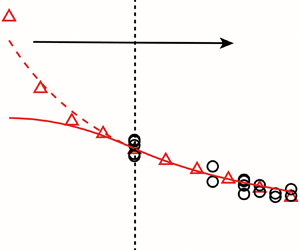
Figure 10. (a) The relationship between parameter $\varepsilon$ and $L/D$ reproduced from Linden & Turner (2001) (the black hollow points), where the red line is the least squares fitting result of the first six points. (b) The relationship between $B(\varepsilon )L/D$ and $L/D$ obtained by bringing the discrete relationship and fitting results in (a), which are shown as black solid points and red hollow points, respectively; the black line is the least squares fitting result of the first six black solid points.

3.4.2. Application of the analytical model to background co-flow ($0< R_v\leq 0.5$)

Based on $\varGamma \sim 1-R_v^2$ from (3.6) for co-flow, (3.21) can be rewritten as

(3.22)\begin{equation} \frac{F_{t^*(R_v>0)}}{F_{t^*(R_v=0)}}=(1+R_v)^{{-}1.5}. \end{equation}

From the previous research on starting jets without background flow (Gharib et al. 1998; Rosenfeld et al. 1998) and the results obtained by the present numerical method for case 1, $F_{t^*(R_v=0)}=4$ can be found. Therefore, $F_{t^*(R_v>0)}=4(1+R_v )^{-1.5}$ can be obtained from (3.22) for the range $0< R_v\leq 0.5$. The results of the model calculation and the results from the present numerical method and the experiment data from Krueger et al. (2006) are shown in figure 11. Equation (3.22) can describe accurately the variation of formation number in the presence of background co-flow for $0< R_v\leq 0.5$.

Figure 11. The relationship between the formation number $F$ and $R_v$ predicted by (3.22) using $F_{t^*(R_v=0)}=4$ for $0< R_v\leq 0.5$.

3.4.3. Application of the analytical model to background counter-flow ($-0.4\leq R_v<0$)

Based on $\varGamma \sim 1+R_v^2$ from (3.6) for counter-flow, (3.21) can be rewritten as

(3.23)\begin{equation} \dfrac{F_{t^*(R_v<0)}}{F_{t^*(R_v=0)}}=\left(\dfrac{1-R_v}{1+R_v^2}\right)^{1.5}. \end{equation}

The predicted results of (3.23) by using $F_{t^*(R_v=0)}=4$ are shown in figure 12 with $F_{t^*}$ in cases 16–19, 21, 22, 24 and 25. The prediction error of (3.23) becomes larger with decreasing $R_v$; nevertheless, it can still indicate qualitatively the trend that the formation number $F_{t^*}$ increases as $R_v$ decreases.

Figure 12. The relationship between the formation number in formation time $t^*$ and $R_v$ predicted by (3.23) in the red solid line and (3.24) in the red dashed line using $F_{t^*(R_v=0)}=4$ for $-0.4\leq R_v<0$.

During the development of this analytical model, the model for $\varGamma$ is more important, as it has exponent $3/2$ in (3.14), compared to the exponent $1/2$ for $I$. However, recall that figure 4, $\varGamma \sim 1+R_v^2$, used to obtain (3.23) holds only for $R_v=-0.1$, while $\varGamma \sim 1-R_v^2$, which is originally used for co-flow ($R_v>0$), seems more suitable for $R_v<-0.1$. This also explains why (3.23) works well only for $R_v=-0.1$. Using $\varGamma \sim 1-R_v^2$ instead of $\varGamma \sim 1+R_v^2$, (3.23) can be rewritten as

(3.24)\begin{equation} \dfrac{F_{t^*(R_v<0)}}{F_{t^*(R_v=0)}}=(1+R_v)^{{-}1.5}, \end{equation}

whose right-hand side is the same as (3.22). The relationship in (3.24) is shown in figure 12 in the form of a red dashed line. It can be seen that (3.24) can capture better the variation of $F_{t^*}$ for $R_v<-0.1$. It can also be concluded that the accurate description of the total jet circulation has a great influence on the final prediction results of this kinematic model. Furthermore, it should be noted that the prediction result of (3.24) still underestimates $F_{t^*}$ at $R_v=-0.4$, as shown in figure 12. On the one hand, the total jet circulation with counter-flow is even smaller than that with co-flow at the same $R_v^2$ ($R_v^2=0.16$) (recall figure 4), which means that $\varGamma \sim 1-R_v^2$ is no longer suitable. On the other hand, the failure of the linear basis $\varepsilon \sim k_1L/D$ and $B(\varepsilon )\,L/D\sim k_2L/D$ used to close this kinematic model when $L/D$ is larger than 7 (figure 10b) may also be the reason for the relatively larger error with the model when $R_v=-0.4$. In general, we can expect that the accurate description model for $\varGamma$ with background counter-flow could help the analytical model developed in the present work to predict the formation number more accurately.

4. Summary

The leading vortex ring formation process with simultaneously initiated uniform background co- and counter-flow has been studied numerically and analytically for $-0.5\leq R_v\leq 0.5$, where $R_v$ is the ratio of background co- or counter-flow velocity to jet velocity. Altogether, 26 different cases have been examined numerically. The results show that the axial displacement of the leading vortex ring at the same formation time will be larger with increasing $R_v$. Using the slug model, the translational velocity of the leading vortex ring in the inertial reference system can be expressed as $U_{in}(1+R_v)/2$, where $U_{in}$ is the jet velocity. A critical velocity ratio ($R_{crit}=-0.4$) has been found for background counter-flow. For $R_v<-0.4$, the leading vortex ring would be confined near the nozzle exit for a longer period or even moving upstream under the action of background counter-flow. This would cause the trailing jet to pass through it (a phenomenon similar to leapfrogging) and destroy the normal formation process of the leading vortex ring in the starting jet.

Quantitative analysis of the influence of background flow has been carried out by calculating the formation number $F_{t^*}$ for cases 1–3, 5–19, 21, 22, 24 and 25. For the range of $R_v$ from $0$ to $0.5$, $F_{t^*}$ decreases from $3.95$ to $1.92$, while it increases from $3.95$ at $R_v=0$ to $9.6$ at $R_v=-0.4$. In addition, as the jet-based Reynolds number $Re_j$ increases from 1016 to 1524, there is minimal variation observed in $F_{t^*}$ of starting jet with background flow.

An analytical model is proposed based on a kinematic criterion that the pinch-off occurs when the self-induced velocity of the leading vortex ring is equal to the velocity of the jet shear layer in the reference system moving with the background flow. The linear relationship between the vortex core parameter and stroke ratio of the starting jet ($\varepsilon \sim k_1L/D$) for the Norbury vortex ring has been used effectively to close the model. For $0< R_v\leq 0.5$, the ratio of $F_{t^*(R_v>0)}$ to $F_{t^*(R_v=0)}$ is $(1+R_v)^{-1.5}$. This relationship is consistent with that obtained by the present numerical method and the experiments by Krueger et al. (2006). For $-0.4\leq R_v<0$, the ratio of $F_{t^*(R_v<0)}$ to $F_{t^*(R_v=0)}$ is $((1-R_v)/(1+R_v^2 ))^{1.5}$. However, the prediction error of this equation increases with decreasing $R_v$ for $R_v<-0.2$. By analysis, this can be attributed to the fact that the circulation model for counter-flow ($\varGamma \sim 1+R_v^2$ from (3.6)) cannot reflect the interaction between the leading vortex ring and the nozzle wall. In contrast, it is found that the relationship between the formation number and $R_v$ derived for co-flow, $F_{t^*(R_v\!{\neq}0)}= F_{t^*(R_v=0)}(1+ R_v)^{-1.5}$, satisfies the range $-0.4\leq R_v\leq -0.2$ more.