Stability theory for metal pad roll in cylindrical liquid metal batteries

Abstract

When liquid metal batteries are charged or discharged, strong electrical currents are passing through the three liquid layers that we find in their interior. This may result in the metal pad roll instability that drives gravity waves on the interfaces between the layers. In this paper, we investigate theoretically metal pad roll instability in idealised cylindrical liquid metal batteries that were simulated previously by Weber et al. (Phys. Fluids, vol. 29, no. 5, 2017b, 054101) and Horstmann et al. (J. Fluid Mech., vol. 845, 2018, pp. 1–35). Near the instability threshold, we expect weakly destabilised gravity waves, and in this parameter regime, we can use perturbation methods to find explicit formulas for the growth rate of all possible waves. This perturbative approach also allows us to include dissipative effects, hence we can locate the instability threshold with good precision. We show that our theoretical growth rates are in quantitative agreement with previous and new direct numerical simulations. We explain how our theory can be used to estimate a lower bound on cell size beneath which metal pad roll instability is unlikely.

1. Introduction

The metal pad roll instability is a well-known phenomenon that causes undesirable wave motion on the cryolite–aluminium interface inside Hall–Héroult reduction cells. Since Sele (1977), we have known that this wave motion is due to a magnetohydrodynamic coupling between the ambient magnetic field and the electrolysis current that is being deflected by the waves. The review of Gerbeau, Le Bris & Lelièvre (2006) contains a rich bibliography on this subject.

Liquid metal batteries are structurally similar to reduction cells but have three layers of stacked fluids (light metal, molten salt, heavy alloy) rather than two (cryolite, aluminium). Existing prototypes of liquid metal batteries (Bradwell et al. 2012; Wang et al. 2014) are certainly not yet as large as industrial reduction cells, but if they were to be made as large in the future, then it is likely that metal pad roll instability will also be present in these batteries and affect their efficiency. Zikanov (2015) is the first to discuss metal pad roll instability in liquid metal batteries. In this paper, the solid-slab model of Davidson & Lindsay (1998) is extended to the three-layer case, which suggests that the physical mechanism causing metal pad instability in batteries is essentially the same as in reduction cells. Shallow-layer magnetohydrodynamic models give a more precise description of the metal pad roll instability and were very popular in the two-layer reduction cell context (see Bojarevics & Romerio 1994; Bojarevics 1998; Davidson & Lindsay 1998; Zikanov et al. 2000; Lukyanov, El & Molokov 2001; Sun, Zikanov & Ziegler 2004; Zikanov, Sun & Ziegler 2004). In Bojarevics & Tucs (2017), Tucs, Bojarevics & Pericleous (2018a,b) and Molokov (2018), we find three-layer extensions of these shallow-layer modes, adapted to large-scale batteries. All these models can find the most unstable mode and how this depends on the type of battery, the materials and also the geometry of the cell. Dissipation is less easily modelled, but should be less important in such large-scale cells. Tucs et al. (2018b) make an interesting numerical application for 10 different metal–salt–alloy combinations that have been used to build liquid metal batteries. Considering a large-scale cell with a design that is close to that of an industrial aluminium reduction cell (8 m by 3.6 m, total current $10^5$ A, metal–salt–alloy heights 20, 4 and 20 cm, respectively), they find from theory that metal pad instability requires no more than $0.1$–$0.6$ mT of vertical magnetic field. This very low critical magnetic field can easily be driven by the power lines that would surround the cells, and confirms that large-scale liquid metal batteries, if they are built as reduction cells, will likely be unstable.

In parallel to the shallow-layer approach, several groups have used direct numerical simulations (DNS) to study metal pad roll instability in three-layer systems. Weber et al. (2017a,b) study a small cylindrical Mg$\|$Sb liquid metal battery using the OpenFOAM code. Many physical parameters (e.g. current, imposed magnetic field, viscosities, densities, fluid layer heights) were varied to see how they affect the instability. The bottom layer of the Mg$\|$Sb battery is so heavy that it almost remains at rest, and as a result, metal pad roll instability is very similar to that found in two-layer reduction cells. Horstmann, Weber & Weier (2018) continue this study and show that other wave types are possible. In the simulations, wave selection depends on the ratio of density jumps $D=(\rho _2- \rho _1)/(\rho _3-\rho _2)$. When $D$ is very different from 1, metal pad roll will be as in a two-layer system. When $D\approx 1$, all three layers are coupled hydrodynamically, and a wave with synchronously rotating top and bottom interfaces is observed. Xiang & Zikanov (2019) present 21 numerical case studies on metal pad roll in cuboid cells. These simulations are also done with OpenFOAM, and the role of the parameter $D$ in selecting different wave patterns is confirmed by this study.

Both shallow-layer models and DNS provide useful information on what metal pad roll instability could look like in liquid metal batteries, but we need to underline that they are describing essentially different cells. Where shallow models are designed for large-scale cells, all the simulated cells in DNS are without exception small, typically some 10 cm in size. DNS does not filter out turbulent fluid motion, and this limits simulations to Reynolds number flows $Re < 10^4$ in practice. With realistic viscosities that are often lower than $10^{-6}\ {\rm m}^2\ {\rm s}^{-1}$, and typical flow magnitudes of just a few cm s$^{-1}$, we are already reaching the interval $Re \in [10^3, 10^4]$ in 10 cm cells. This explains why all simulations are done in small cells. Qualitatively, metal pad roll instability is similar in shallow models and DNS, but quantitatively, we can expect significant differences. The small cells in DNS are rarely shallow and also much more prone to viscous dissipation. In small cells, a larger magnetic field needs to be imposed in order to trigger the metal pad roll instability, in which case inductive currents can also cause an extra magnetic damping (Sreenivasan, Davidson & Etay 2005). A stability theory that matches quantitatively with DNS of small cells needs to be non-shallow and it needs to include a precise description of dissipative effects.

The previous observations have motivated us to run a research programme on metal pad roll instability in two- and three-layer systems, in which we seek for common ground between stability theory and DNS. Our focus is on cylindrical cells that have been studied before by Weber et al. (2017a,b) and Horstmann et al. (2018). We can simulate these cells with two different numerical solvers, OpenFOAM and SFEMaNS (see Guermond et al. 2007, 2009; Nore et al. 2016; Cappanera et al. 2018). The cylindrical geometry also greatly simplifies the stability theory with respect to the case of rectangular section cells. In Herreman et al. (2019) (referred to as H19 in what follows) we derived the two-layer stability theory. The idea is that near the threshold of the metal pad roll instability, the Lorentz force is weakly destabilising the free gravity waves. Using standard perturbation methods, we can model the effect of the Lorentz force and viscous dissipation perturbatively. This results in an explicit formula for the growth rate that should be valid near the threshold. In H19, we quantitatively validated this theory by comparing numerically measured growth rates from DNS to the theory. In Nore et al. (2021), we modified the two-layer theory to show that metal pad roll instability in a small centimetre scale experiment that places gallium over mercury is possible. This new paper is our third contribution on the subject of metal pad roll instability, and it extends our perturbative stability theory to three-layer liquid metal batteries.

The paper is structured as follows. In § 2, we present the stability theory, following the same steps as in H19. In § 3, we apply the theory to different cylindrical liquid metal battery models. In § 3.1, we apply the theory to the Mg$\|$Sb cell of Weber et al. (2017a,b) and show quantitative agreement with DNS. In § 3.2, we apply the theory to the three-layer set-ups simulated by Horstmann et al. (2018). Our theory indeed suggests that we can have both types of symmetrical and antisymmetrical waves as the most unstable wave, and that this depends on the density jump ratio $D$. In the vicinity of $D \approx 1$, we also find that metal pad roll instability in three-layer systems may be very weak, because the Lorentz force can be locally stabilising in one fluid layer and locally destabilising in another. This is a peculiarity of metal pad roll in three-layer systems that has no two-layer equivalent. Tucs et al. (2018a) have studied metal pad roll in a small square Na$\|$Bi cell using a shallow model, and in § 3.3, we apply our theory to a cylindrical analogue of this square cell. According to our theory, this cell is much less unstable, and this is also confirmed by a challenging numerical simulation. In § 3.4, we take inspiration from Tucs et al. (2018b) and compute the critical magnetic fields $B_{z,c}$ for the onset of instability in a hypothetical $10^5$ A cylindrical cell. We find very similar critical magnetic fields for the onset of instability. Finally, in § 3.5, we map the domain of stability of different types of batteries in a size of cell versus current density chart and in a worst case scenario. Using this type of figure, we can give a lower bound on the battery size that is needed to find metal pad roll instability.

2. Metal pad roll stability theory

2.1. Base state

We model metal pad roll (MPR) instability in an idealised three-layer cylindrical liquid metal battery (LMB). We use the notations of figure 1(a), which shows the base state that we assume in our model. The cylinder has radius $R$, and the heights of the three layers are $H_i$, with $i=1,2,3$. We use cylindrical coordinates $(r,\theta,z)$ and basis $(\boldsymbol {e}_r,\boldsymbol {e}_{\theta },\boldsymbol {e}_z)$. The electrical conductivity, density and kinematic viscosity are denoted $\sigma _i$, $\rho _i$ and $\nu _i$ in layers $i=1,2,3$. We will denote density differences as

(2.1a,b)\begin{equation} \Delta \rho_{12} = \rho_2 - \rho_1, \quad \Delta \rho_{23} = \rho_3 - \rho_2, \end{equation}

Standard gravity is $g$, and we ignore surface tension in this study. We assume a base state with all fluids at rest separated by planar interfaces at $z=0$ ($1|2$ interface) and $z=-H_2$ ($2|3$ interface). The base state pressure $P_i$ is hydrostatic, $\partial _z P_i = - \rho _i g$, and continuous at the interfaces, so $(P_1,P_2,P_3)=P_0 + (-\rho _1 gz, - \rho _2 g z , - \rho _3 g (z + H_2) + \rho _2 g H_2)$, with $P_0$ denoting an arbitrary ambient pressure. We have solid electrodes connecting to the liquids at $z=H_1$ and $z=-H_2 - H_3$, with an electrical conductivity that is supposed significantly smaller compared to that of the liquid metals in zones $1$ and $3$. A perfectly homogeneous electrical current with density $\boldsymbol {J}=J\boldsymbol {e}_z$ runs vertically through the three layers. The base-state electrical potential $\varPhi _i$ is defined by $J = - \sigma _i\, \partial _z \varPhi _i$ and is continuous at the interfaces. This yields $(\varPhi _1 , \varPhi _2, \varPhi _3) = \varPhi _0 + J ( - \sigma _1^{-1} z ,- \sigma _2^{-1} z , - \sigma _3^{-1} (z + H_2) + \sigma _2^{-1} H_2 )$ inside the cell, with $\varPhi _0$ arbitrary. A uniform vertical magnetic field $\boldsymbol {B}^e =B_z\boldsymbol {e}_z$ is applied externally to the cell, and the total magnetic field is $\boldsymbol {B}= (\mu _0 J r/2 )\boldsymbol {e}_\theta + B_z \boldsymbol {e}_z$. In the following, we refer to the unperturbed fluid volumes as $\mathcal {V}_1 , \mathcal {V}_2, \mathcal {V}_3$. The boundaries of these fluid domains are $\delta \mathcal {V}_1 , \delta \mathcal {V}_2,\delta \mathcal {V}_3$ and include the solid walls $\varSigma _1, \varSigma _2 , \varSigma _3$, and the interfaces $z=0$ and $z=-H_2$ are $\mathcal {S}_{12}$ and $\mathcal {S}_{23}$.

Figure 1. Sketch of the base state under study. (a) Three liquid layers with different electrical conductivity, density and kinematic viscosity are stacked stably on top of each other due to gravity. A homogeneous current density $J$ runs vertically through the layers and creates an azimuthal magnetic field $B_\theta$. A uniform vertical magnetic field $B_z$ is applied externally. (b) Our three fluid domains $\mathcal {V}_1,\mathcal {V}_2, \mathcal {V}_3$ have respective heights $H_1,H_2,H_3$ and radius $R$. The solid boundaries are referred to as $\varSigma _1, \varSigma _2 , \varSigma _3$, and the interfaces as $\mathcal {S}_{12}$ and $\mathcal {S}_{23}$.

2.2. Linear perturbation problem

We are interested in the linear stability of the base state defined previously. We denote by $\boldsymbol {u}_i$, $p_i$, $\boldsymbol {b}_i$, $\boldsymbol {j}_i$ and $\varphi _i$ the linear perturbations of flow, pressure, magnetic field, current density and electrical potential, respectively. We assume that the quasi-static limit of magnetohydrodynamics is adequate. A necessary condition is that $\sigma _i \mu _0 \omega R^2 \ll 1$ in all three layers. Here, $\omega$ is any typical frequency of the flow or magnetic field and will be the typical gravity wave frequency in our theory. This inequality is well satisfied in all our applications. The linearised magnetohydrodynamic equations for the perturbations are

(2.2a)$$\begin{gather} \rho_i\,\partial_t\boldsymbol{u}_i+\boldsymbol{\nabla} p_i = \boldsymbol{J}\times\boldsymbol{b}_i+\boldsymbol{j}_i\times\boldsymbol{B}+\rho_i\nu_i\,{\Delta}\boldsymbol{u}_i, \end{gather}$$

(2.2b)$$\begin{gather}\boldsymbol{\nabla} \boldsymbol{\cdot} \boldsymbol{u}_i = 0, \end{gather}$$

(2.2c)$$\begin{gather}\boldsymbol{j}_i = \sigma_i(-\boldsymbol{\nabla} \varphi_i+\boldsymbol{u}_i \times \boldsymbol{B}), \end{gather}$$

(2.2d)$$\begin{gather}\boldsymbol{\nabla} \boldsymbol{\cdot} \boldsymbol{j}_i = 0. \end{gather}$$

The magnetic field perturbation $\boldsymbol {b}_i$ satisfies $\boldsymbol {\nabla } \times \boldsymbol {b}_i=\mu _0\ \boldsymbol {j}_i$ and $\boldsymbol {\nabla } \boldsymbol {\cdot } \boldsymbol {b}_i=0$, but we will not need to calculate this field explicitly. We use the following hydrodynamical boundary conditions. Fluid adheres on the solid wall of the cylinder, so

(2.3a)\begin{equation} \boldsymbol{u}_i = \boldsymbol{0} |_{\varSigma_i}. \end{equation}

We locate the deformed interfaces at $z=\eta _{12} (r,\theta,t)$ and $z=\eta _{23} (r,\theta,t)$. The linearised kinematic boundary conditions that apply at these interfaces are

(2.3b)$$\begin{gather} \partial_t\eta_{12} = u_{1,z}|_{z=0} , \quad \partial_t\eta_{12} =u_{2,z}|_{z=0}, \end{gather}$$

(2.3c)$$\begin{gather}\partial_t\eta_{23} = u_{2,z}|_{z={-}H_2} , \quad \partial_t\eta_{23}=u_{3,z}|_{z={-}H_2}. \end{gather}$$

In viscous fluids, we must also require that tangential flow is continuous at the interface:

(2.3d)$$\begin{gather} {u}_{1,r} |_{z=0} = {u}_{2,r} |_{z=0} , \quad {u}_{1,\theta} |_{z=0} = {u}_{2,\theta} |_{z=0}, \end{gather}$$

(2.3e)$$\begin{gather}{u}_{2,r} |_{z={-}H_2} = {u}_{3,r} |_{z={-}H_2} , \quad {u}_{2,\theta} |_{z={-}H_2} = {u}_{3,\theta} |_{z={-}H_2}. \end{gather}$$

The dynamic boundary conditions express the continuity of stress at the interface. From the normal component, we derive that

(2.3f)$$\begin{gather} \Delta \rho_{12}\,g\eta_{12} + 2 \rho_2 \nu_2\,\partial_z u_{z,2} |_{z=0} - 2 \rho_1 \nu_1\,\partial_z u_{z,1} |_{z=0} = p_2|_{z=0}-p_1|_{z=0}, \end{gather}$$

(2.3g)$$\begin{gather}\Delta \rho_{23}\,g\eta_{23} + 2 \rho_3 \nu_3\,\partial_z u_{z,3} |_{z={-}H_2} - 2 \rho_2 \nu_2\,\partial_z u_{z,2} |_{z={-}H_2} = p_3|_{z={-}H_2}-p_2|_{z={-}H_2}, \end{gather}$$

and from the tangential components,

(2.3h)$$\begin{gather} \rho_1 \nu_1\,\partial_z {u}_{1,r} |_{z=0} = \rho_2 \nu_2\,\partial_z {u}_{2,r} |_{z=0},\quad \rho_1 \nu_1\,\partial_z {u}_{1,\theta} |_{z=0} = \rho_2 \nu_2\, \partial_z {u}_{2,\theta} |_{z=0}, \end{gather}$$

(2.3i)$$\begin{gather}\rho_2 \nu_2\,\partial_z {u}_{2,r} |_{z={-}H_2} = \rho_3 \nu_3\,\partial_z {u}_{3,r} |_{z={-}H_2},\quad \rho_2 \nu_2\,\partial_z {u}_{2,\theta} |_{z={-}H_2} = \rho_3 \nu_3\,\partial_z {u}_{3,\theta} |_{z={-}H_2}. \end{gather}$$

Electrical boundary conditions on the solid walls are

(2.4)\begin{equation} \boldsymbol{j}_i\boldsymbol{\cdot}\boldsymbol{n}_i=0|_{\varSigma_i}. \end{equation}

Here, $\boldsymbol {n}_i$ is the unit normal. This relation is exact on the isolating radial sidewall. It is also a good approximation on the top and bottom lids, $z=H_1$ and $z=-H_2-H_3$, if we assume that solid electrodes above layer 1 and under layer 3 have an electrical conductivity that is significantly lower than $\sigma _1$ and $\sigma _3$ of the metals. Similar assumptions were made in previous shallow-layer models (Molokov 2018; Tucs et al. 2018a,b) and simulations (Weber et al. 2017a,b; Horstmann et al. 2018). At the interfaces, we express that the total normal electrical current $(\boldsymbol {J} + \boldsymbol {j} ) \boldsymbol {\cdot } \boldsymbol {n}$ and total electrical potential $\varPhi +\varphi$ are continuous. After linearisation, this yields

(2.5a)$$\begin{gather} j_{2,z}|_{z=0}-j_{1,z}|_{z=0} = 0, \end{gather}$$

(2.5b)$$\begin{gather}j_{3,z}|_{z={-}H_2}-j_{2,z}|_{z={-}H_2} = 0, \end{gather}$$

(2.5c)$$\begin{gather}\varphi_2|_{z=0}-\varphi_1|_{z=0} = J(\sigma_2^{{-}1}-\sigma_1^{{-}1})\eta_{12}, \end{gather}$$

(2.5d)$$\begin{gather}\varphi_3|_{z={-}H_2}-\varphi_2|_{z={-}H_2} = J(\sigma_3^{{-}1}-\sigma_2^{{-}1})\eta_{23}. \end{gather}$$

Notice here how the surface elevations $\eta _{12} , \eta _{23}$ cause jumps in the electrical potential perturbation $\varphi$ when the conductivities of the layers are different. This physical ingredient is essential for MPR instability. The magnetic field boundary conditions are not so relevant as we will not need to compute $\boldsymbol {b}_i$.

The linear stability problem is now defined entirely. We may search for solutions in which arbitrary field components $f$ grow as $f=\hat {f}e^{st}$. In the following, hatted variables ($\hat {f}$) always represent the spatial structure of a field, $s \in \mathbb {C}$ is named complex growth rate, and instability requires $\mbox {Re} (s) > 0$. As in H19, we choose to not non-dimensionalise the stability problem because there are too many physical parameters.

2.3. Instability mechanism in three-layer systems

Before calculating the growth rate, we discuss the physics of the instability mechanism. In figure 2, we consider a gravity wave that rotates as indicated by the black arrow. The instantaneous interface deformation can be of three different, typical types. In case (a), called the decoupled case by Horstmann et al. (2018), the wave leaves the lower interface mainly undeformed. This situation is the common one in most batteries, because we often have $\Delta \rho _{12} \ll \Delta \rho _{23}$. In some batteries, we can have $\Delta \rho _{12} \approx \Delta \rho _{23}$, and both interfaces will then deform similarly. We can have either (b) antisymmetrically deformed interfaces or (c) symmetrically deformed interfaces.

Figure 2. Metal pad roll instability mechanism in batteries, in three characteristic situations. The top diagrams show interface deformations, instantaneous flows for a rotating wave and current deflections. The bottom diagrams show perturbed current loops and compare the direction of Lorentz force $\boldsymbol {j} \times \boldsymbol {B}^e$ to that of $\boldsymbol {u}$. In many LMBs, $\Delta \rho _{12} \ll \Delta \rho _{23}$, and we expect a waveform as in (a) where the bottom interface remains almost flat. When $\Delta \rho _{23} \approx \Delta \rho _{12}$, other waveforms are possible: (b) antisymmetrical waveforms, or (c) symmetrical waveforms.

In the top diagrams of figure 2, we draw the instantaneous flow, $\boldsymbol {u}$, using green arrows. To understand the direction of $\boldsymbol {u}$, just imagine how fluid material will be displaced when the wave is rotating in the direction of the black arrow. The red arrows of varying thickness suggest the spatial variation of total electrical current, $\boldsymbol {J} + \boldsymbol {j}$. Since the electrolyte is a bad conductor, the current will be intensified (thicker arrows) near the shallower parts of the electrolyte, and weakened (thinner arrows) near the thicker parts of the electrolyte.

In the bottom diagrams of figure 2, we suggest the typical loops associated with the current deviation $\boldsymbol {j}$. In cases (a) and (b), we expect a single $\boldsymbol {j}$ loop, but in case (c), we will rather have a pair of $\boldsymbol {j}$ loops to be able to create a small horizontal current deviation defect within the inclined electrolyte layer. Having these loops in mind, we can now draw the instantaneous direction of the Lorentz force, $\boldsymbol {j} \times \boldsymbol {B}^e$ (light green arrows). If the Lorentz force is to be destabilising, then it has to align more or less with the instantaneous flow as $\boldsymbol {u} \boldsymbol {\cdot } (\,\boldsymbol {j} \times \boldsymbol {B}^e) > 0$ indeed indicates that the wave is being powered electromagnetically. This power injection is obviously very different in cases (a), (b) and (c) according to the sketch.

Let us discuss case (a) first. Figure 2 suggests that $\boldsymbol {u}$ aligns with $\boldsymbol {j} \times \boldsymbol {B}^e$ in the top layer, so the wave is being powered by the Lorentz force in this layer. As the same figure can be drawn at any rotated position, we can expect a permanent injection of power and hence a permanent electromagnetic amplification. In this battery type with $\Delta \rho _{12} \ll \Delta \rho _{23}$, the bottom layer is almost at rest, and hence with $\boldsymbol {u}_3 \approx \boldsymbol {0}$, this layer will not be receiving much power from the Lorentz force. The result is that MPR will be very much as in a two-layer system, and we already know that this is true from the simulations of Weber et al. (2017a,b) of Mg$\|$Sb batteries. Notice finally that the direction of rotation of the wave is crucial for amplification. If we invert the rotation direction, then $\boldsymbol {u}$ changes sign and hence anti-aligns with $\boldsymbol {j} \times \boldsymbol {B}^e$. The wave rotating in the opposite direction would be electromagnetically damped.

When $\Delta \rho _{12} \approx \Delta \rho _{23}$, other waveforms are possible, as we know from Horstmann et al. (2018), and power injection will also be rather different in this situation. On the typical $\boldsymbol {j}$ loops, it is easy to draw the instantaneous direction of the Lorentz force $\boldsymbol {j} \times \boldsymbol {B}^e$, and this has been done in the sketch. Interestingly, it seems that $\boldsymbol {u} \boldsymbol {\cdot } (\,\boldsymbol {j} \times \boldsymbol {B}^e) > 0$ in the top layer, but that $\boldsymbol {u} \boldsymbol {\cdot } (\,\boldsymbol {j} \times \boldsymbol {B}^e) < 0$ in the bottom layer, for both symmetrical and antisymmetrical waveforms. What this suggests is that energy may be injected into a rotating wave in one layer (top), but that at the same time, energy will be withdrawn from the wave in the other layer (bottom). This situation of opposing power transfers is obviously a peculiarity of the MPR instability in three-layer systems and of these symmetrical or antisymmetrical waveforms. It also seems to suggest that with $\Delta \rho _{12} \approx \Delta \rho _{23}$, we can end up with a situation where as much electromagnetic power is being injected as there is electromagnetic power being withdrawn. This seems to suggest that MPR instability can be very weak when $\Delta \rho _{12} \approx \Delta \rho _{23}$. We will see that our stability analysis confirms this idea.

In the previous diagrams, we have considered only the vertical, external magnetic field $\boldsymbol {B}^{e} = B_z \boldsymbol {e}_z$, but it is instructive to make similar diagrams using the azimuthal magnetic field $B_\theta = \mu _0 J r/2$. This allows us to see that the Lorentz force $\boldsymbol {j} \times (B_\theta \boldsymbol {e}_\theta )$ never really aligns with the instantaneous wave flow, which suggests that the azimuthal magnetic field cannot cause electromagnetic amplification of gravity waves. Our theory confirms this suggestion. The azimuthal field can only change the frequency of the waves, but it will never amplify them, just as in two-layer systems (see H19 and Sneyd 1985; Sneyd & Wang 1994).

2.4. Perturbative solution

We now come to the main objective in this linear stability problem: the calculation of the complex growth rate $s$ of different wave modes. We apply the perturbative method of H19 to the three-layer case. Let us recall the general idea. Near the instability threshold, when the Lorentz force is sufficiently small compared to pressure and inertia, we can expect that the unstable modes will be weakly perturbed rotating gravity waves. Near the threshold, the complex growth rate of a rotating wave will be

(2.6)\begin{equation} s = \mathrm{i} \omega + \underbrace{ \lambda + \mathrm{i} \delta }_{\text{small shift}}. \end{equation}

Here, $\omega$ is the frequency of the free inviscid gravity wave. Small viscosity and small Lorentz forces cause a small complex shift of the eigenvalue $\mathrm {i} \omega$, which we split into a real and an imaginary part as $\lambda + \mathrm {i}\delta$. The quantity $\delta$ captures a real frequency shift, and we will not calculate it explicitly, since it has no impact on the stability of the wave. We will rather focus on the real growth rate $\lambda$ that is further split into three independent terms:

(2.7)\begin{equation} \lambda=\lambda_v+\lambda_{vv} + \lambda_{visc}. \end{equation}

In this formula, the Lorentz force creates the terms $\lambda _v$ and $\lambda _{vv}$, and the viscous force creates the correction $\lambda _{visc}$. We have this additive structure because both types of forces are considered as weak independent perturbations in the model. The term $\lambda _v \sim JB_z$ is the only one that can be positive, and it relates to the instability mechanism that was discussed in the previous subsection. The term $\lambda _{vv} < 0$ is the weak magnetic damping due to induction in the top and bottom metals. Proportional to $B_z^2$, it is very small for low imposed magnetic fields. The term $\lambda _{visc} < 0$ is the viscous damping of the wave. This damping is due to dissipation in the thin Stokes layers that exist at the solid boundaries and near the $1|2$ and $2|3$ interfaces.

In the following subsections, we calculate $\lambda _v$, $\lambda _{vv}$, $\lambda _{visc}$ by taking the following steps. In § 2.4.1, we solve the unperturbed wave problem: we calculate the spatial structure and frequency $\omega$ of free inviscid gravity waves in the three-layer system. In § 2.4.2, we formulate sufficient conditions to use perturbation methods: we estimate when the Lorentz and viscous forces are small compared to pressure forces and inertia. In § 2.4.3, we solve the electrical problem in the electrostatic limit: we find the dominant part of the electrical current perturbation that is caused by the interface elevations created by the waves. In § 2.4.4, we compute the growth rate $\lambda _v$ of instability in the dissipationless limit using a perturbative expansion and a solvability condition. In § 2.4.5, we compute the magnetic damping correction $\lambda _{vv}$ that is due to inductive corrections in Ohm's law. In § 2.4.6, we calculate the viscous damping correction $\lambda _{visc}$. We identify the Stokes boundary layer structure and compute dissipation therein.

Once everything is computed, we can better estimate the domain of applicability of the theory. What we really need to have in the perturbative limit is a small shift in the eigenvalue, meaning that

(2.8a–c)\begin{equation} \left| \frac{\lambda_v }{\omega} \right| \ll 1 , \quad \left| \frac{\lambda_{vv} }{\omega} \right| \ll 1 , \quad \left| \frac{\lambda_{visc} }{\omega} \right| \ll 1, \end{equation}

are necessary. In all the numerical applications of § 3, we satisfy these inequalities.

2.4.1. First step: unperturbed wave problem

The perturbative approach starts with a characterisation of the leading-order inviscid hydrodynamical wave problem. We will denote these wave solutions as

(2.9)\begin{equation} [\boldsymbol{u}_i,p_i,\eta_{12},\eta_{23}]=[\hat{\boldsymbol{u}}_i, \hat{p}_i,\hat{\eta}_{12},\hat{\eta}_{23}]\, {\rm e}^{\mathrm{i}\omega t}, \end{equation}

using hatted variables for the spatial structure, and $\omega$ for the inviscid frequency. Without Lorentz and viscous forces, we need to solve

(2.10a) \begin{equation} \rho_i (\mathrm{i} \omega) \hat{\boldsymbol{u}}_i+\boldsymbol{\nabla} \hat{p}_i=0, \quad \boldsymbol{\nabla} \boldsymbol{\cdot} \hat{\boldsymbol{u}}_i=0, \end{equation}

with the inviscid limit of the boundary conditions (2.3), $\hat {\boldsymbol {u}}_i \boldsymbol {\cdot } \boldsymbol {n}_i = {0} |_{\varSigma _i}$ on the solid walls, and

(2.10b)$$\begin{gather} \mathrm{i} \omega \hat{\eta}_{12} = \hat{u}_{1,z}|_{z=0} =\hat{u}_{2,z}|_{z=0} , \quad \mathrm{i} \omega \hat{\eta}_{23}=\hat{u}_{2,z}|_{z={-}H_2} =\hat{u}_{3,z}|_{z={-}H_2}, \end{gather}$$

(2.10c)$$\begin{gather}\Delta \rho_{12}\,g\hat{\eta}_{12} = \hat{p}_2|_{z=0}-\hat{p}_1|_{z=0} , \quad \Delta \rho_{23}\,g \hat{\eta}_{23} =\hat{p}_3|_{z={-}H_2}-\hat{p}_2|_{z={-}H_2} \end{gather}$$

on the interfaces. This three-layer wave problem was already studied in detail by Horstmann et al. (2018). We use slightly different notations to remain as close as possible to the presentation of H19 that we wish to extend. The flow is potential: $\hat {\boldsymbol {u}}_i=\boldsymbol {\nabla } \hat {\phi }_i$ and $\nabla ^2 \hat {\phi }_i=0$. We find the hydrodynamic potentials and the interface deformations as

(2.11a)$$\begin{gather} \hat{\phi}_1 = \frac{\omega R}{k}\, a\,\frac{\cosh(k(z-H_1))}{\sinh(kH_1)}\,J_m(kr)\, {\rm e}^{\mathrm{i} m\theta}, \end{gather}$$

(2.11b)$$\begin{gather}\hat{\phi}_2 = \frac{\omega R}{k}\left(b\,\frac{\cosh(kz)}{\sinh(kH_2)} -a\,\frac{\cosh(k(z+H_2))}{\sinh(kH_2)}\right)J_m(kr)\, {\rm e}^{\mathrm{i} m\theta}, \end{gather}$$

(2.11c)$$\begin{gather}\hat{\phi}_3 ={-} \frac{\omega R}{k} \, b\,\frac{\cosh(k(z+H_2+H_3))}{\sinh(kH_3)}\,J_m(kr)\, {\rm e}^{ \mathrm{i} m\theta}, \end{gather}$$

and

(2.11d)$$\begin{gather} \hat{\eta}_{12} = R \mathrm{i} a\,J_m(kr)\, {\rm e}^{\mathrm{i} m\theta}, \end{gather}$$

(2.11e)$$\begin{gather}\hat{\eta}_{23} = R \mathrm{i} b\,J_m(kr)\, {\rm e}^{\mathrm{i} m\theta}. \end{gather}$$

Pressure relates to hydrodynamic potential by $\hat {p}_i = -\mathrm {i} \omega \rho _i \hat {\phi }_i$. In these formulas, $J_m$ represents a Bessel function of the first kind, $m\in \mathbb {N}$ is the azimuthal wavenumber that can be considered positive, and $k$ is the radial wavenumber that takes the discrete values $k=\kappa _{mn}/R$, with $\kappa _{mn}$ the $n$th zero of $J'_m(\kappa _{mn})=0$. The solution (2.11) satisfies impermeability on the solid walls and the kinematic boundary conditions on the interfaces. The non-dimensional amplitudes $a,b$ are still undetermined, but they are non-trivially related by the algebraic system that is found by expressing the dynamic boundary conditions (2.3f) and (2.3g) as

(2.12) \begin{equation} \begin{pmatrix} \dfrac{\omega_{12}^2}{\omega^2} - 1 & \dfrac{ \rho_2 }{\bar{\rho}_{12} \sinh(kH_2)} \\ \dfrac{ \rho_2 }{\bar{\rho}_{23} \sinh(kH_2)} & \dfrac{\omega_{23}^2}{\omega^2} - 1 \end{pmatrix} \begin{pmatrix} a \\ b \end{pmatrix} = \begin{pmatrix} 0 \\ 0 \end{pmatrix}. \end{equation}

Henceforth, we use the notation

(2.13a)$$\begin{gather} \bar{\rho}_{12}=\frac{\rho_1}{\tanh(kH_1)}+\frac{\rho_2}{\tanh(kH_2)}, \quad \bar{\rho}_{23}=\frac{\rho_2}{\tanh(kH_2)} + \frac{\rho_3}{\tanh(kH_3)}, \end{gather}$$

(2.13b)$$\begin{gather}\omega_{12}^2=\frac{ \Delta \rho_{12}\,gk}{\bar{\rho}_{12}} , \quad \omega_{23}^2=\frac{\Delta \rho_{23}\,gk}{\bar{\rho}_{23}}. \end{gather}$$

The frequencies $\omega _{12}$ and $\omega _{23}$ are the wave frequencies of the respective two-layer systems. Existence of non-trivial solutions of (2.12) requires that

(2.14)\begin{equation} \left[\frac{1}{\omega^2}-\frac{1}{\omega^2_{12}}\right] \left[\frac{1}{\omega^2}-\frac{1}{\omega^2_{23}}\right]= \frac{\rho^2_2}{\bar{\rho}_{12}\bar{\rho}_{23}\sinh^2(kH_2)\, \omega_{12}^2\omega_{23}^2}, \end{equation}

from which we can find that there are two possible values of $\omega ^2$:

(2.15)\begin{align} \omega_\pm^2 = \left( \frac{1}{2}\left(\frac{1}{\omega^2_{12}}+\frac{1}{\omega^2_{23}}\right) \mp \frac{1}{2} \sqrt{\left(\frac{1}{\omega^2_{12}}-\frac{1}{\omega^2_{23}}\right)^2+ \frac{4}{\omega^2_{12}\omega^2_{23}}\, \frac{\rho^2_2}{\bar{\rho}_{12}\bar{\rho}_{23}}\,\frac{1}{ \sinh^2(kH_2) }} \right)^{{-}1}. \end{align}

The sign $\pm$ chooses between the rapid frequency ($+$) branch and the slow frequency ($-$) branch, and here we use the same notation as in Horstmann et al. (2018). Returning these two possible values of $\omega ^2$ to the original system (2.12), we find unique amplitude ratios $\epsilon = b / a$ for both the slow and rapid branches:

(2.16a)\begin{equation} \epsilon_\pm{=} C \pm \sqrt{C^2+D}, \end{equation}

with

(2.16b)\begin{equation} C=\frac{1}{2}\left(\frac{\bar{\rho}_{12}}{\rho_2}-\frac{\Delta \rho_{12}}{\Delta \rho_{23}}\,\frac{\bar{\rho}_{23}}{\rho_2}\right)\sinh(kH_2) , \quad D= \frac{\Delta \rho_{12}}{\Delta \rho_{23}}. \end{equation}

Fast waves always have $\epsilon _+ > 0$: both interfaces deform in phase, and have their maxima and minima at the same azimuthal angle $\theta$. This waveform is referred to as symmetrical in Horstmann et al. (2018). Slow waves always have $\epsilon _- < 0$: both interfaces deform in phase opposition. Troughs of the upper $1|2$ interface will be right above crests of the lower $2|3$ interface. This waveform is referred to as antisymmetrical in Horstmann et al. (2018). The difference is illustrated visually in figure 3 for the fundamental slow and fast waves that have $m=1$ and $n=1$.

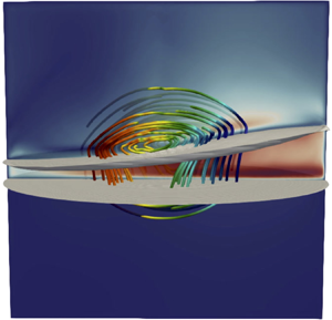
Figure 3. Illustration of the typical interface deformation for a rotating $(1,1,\pm )$ wave. The green arrows suggest a positive rotation direction for a wave with $\omega <0$. Top and bottom interface deformations are (a) in phase opposition for slow $-$ waves, with the amplitude ratio $\epsilon _- < 0$. For rapid $+$ waves, they are (b) in phase, with the amplitude ratio $\epsilon _+ >0$.

In the following, we will refer to a particular wave by providing the triplet $(m,n,\pm )$. For each triplet $(m,n,\pm )$, we have unique values of $\omega _\pm$ and $\epsilon _\pm$. The frequency $\omega$ itself can take four values, $+\omega _-,-\omega _-, +\omega _+,-\omega _+$, and the sign of this frequency carries information on the direction of rotation of the wave. By convention, we fix $m>0$, and by definition, all field profiles are proportional to $\exp ( {\rm i} (m \theta + \omega t))$. Hence with $\omega < 0$ we have a wave that rotates in the positive $+\boldsymbol {e}_\theta$ direction. In figure 3, this rotation direction is suggested by the green arrows.

2.4.2. Second step: sufficient conditions that allow the use of perturbation methods

Near the threshold of instability, when Lorentz forces ($\boldsymbol {J}\times \boldsymbol {b}_i+\boldsymbol {j}_i\times \boldsymbol {B}$) and viscous forces ($\rho _i\nu _i\,{\Delta }\boldsymbol {u}_i$) are small in comparison to inertia and pressure forces ($\rho _i\partial _t \boldsymbol {u}_i$ and $\boldsymbol {\nabla } p_i$), we can model their effect on the waves perturbatively. Using the same order of magnitude analysis as in H19 (§ 2.5), not repeated here, we can delimit this perturbative parameter regime by expressing that the inequalities

(2.17a–e)\begin{equation} \frac{\nu_i}{\omega R^2} \ll 1 , \quad \frac{\mu_0 J^2}{\rho_i \omega^2 } \ll 1 , \quad \frac{\mu_0 \sigma_i JR B }{\rho_i \omega } \ll 1 , \quad \frac{JB }{\rho_i \omega^2 R } \ll 1 , \quad \frac{\sigma_i B^2 }{\rho_i \omega^2 R } \ll 1 \end{equation}

need to be satisfied in all three layers $i=1,2,3$, and with $B=B_z$ or $\mu _0 J R$. This set of conditions is to be interpreted only as qualitative, sufficient conditions. More precise conditions can be formulated only a posteriori, by expressing the inequalities (2.8a–c).

2.4.3. Third step: electrical problem in the electrostatic limit

If we consider the Lorentz force as a small perturbation in the momentum balance, then the leading-order hydrodynamical problem has the purely hydrodynamical waves as solutions. These waves cause a redistribution of electrical current that we need to compute. In this subsection, we find the dominant part of the current perturbation that is due to interface deformation (boundary conditions (2.5c) and (2.5d)). This can be done using a static approximation of Ohm's law that ignores the inductive term ($\sigma _i \boldsymbol {u}_i \times \boldsymbol {B}$). In § 2.4.5, we will identify the much smaller electrical current corrections that are due to induction.

We write $[\,\boldsymbol {j}_i,\varphi _i]= [\,\hat {\boldsymbol {j}}_i,\hat {\varphi }_i ]\, {\rm e}^{\mathrm {i}\omega t}$. The spatial structures of these fields need to satisfy

(2.18a,b)\begin{equation} \hat{\boldsymbol{j}}_i={-}\sigma_i\,\boldsymbol{\nabla} \hat{\varphi}_i \quad \boldsymbol{\nabla} \boldsymbol{\cdot} \hat{\boldsymbol{j}}_i=0, \end{equation}

together with all boundary conditions (2.4) and (2.5), expressed in terms of hatted variables. We find the electrical potential solutions as

(2.19a)$$\begin{gather} \hat{\varphi}_1 = \frac{JR}{\sigma_1}\,c\,\frac{\cosh(k(z-H_1))}{\sinh(kH_1)}\,J_m(kr)\, {\rm e}^{{\rm i} m\theta}, \end{gather}$$

(2.19b)$$\begin{gather}\hat{\varphi}_2 =\frac{JR}{\sigma_2}\left(d\,\frac{\cosh(kz)}{\sinh(kH_2)} -c\,\frac{\cosh(k(z+H_2))}{\sinh(kH_2)}\right)J_m(kr)\, {\rm e}^{{\rm i} m\theta}, \end{gather}$$

(2.19c)$$\begin{gather}\hat{\varphi}_3 ={-}\frac{JR}{\sigma_3}\,d\,\frac{\cosh(k(z+H_2+H_3))}{\sinh(kH_3)}\,J_m(kr)\, {\rm e}^{{\rm i} m\theta}. \end{gather}$$

All electrical boundary conditions on the solid walls are built-in, and one can check that $j_z$ is indeed continuous at $z=0$ and $z=-H_2$. The coefficients $c,d$ are still undetermined, but they are related to $a,b$ by the algebraic equations that follow from the jump conditions on the electrical potential perturbations (2.5):

(2.20a) \begin{equation} \begin{pmatrix} -A_{12} & ( \sigma_2 \sinh(kH_2) )^{{-}1}\\ (\sigma_2 \sinh(kH_2) )^{{-}1} & -A_{23} \end{pmatrix} \begin{pmatrix} c \\ d \end{pmatrix} = \begin{pmatrix} \mathrm{i} (\sigma_2^{{-}1} - \sigma_1^{{-}1} ) a \\ \mathrm{i} (\sigma_3^{{-}1} - \sigma_2^{{-}1} ) b \end{pmatrix}. \end{equation}

Here, we note

(2.20b)$$\begin{gather} A_{12} = \sigma_1^{{-}1} \tanh^{{-}1}(kH_1)+\sigma_2^{{-}1} \tanh^{{-}1}(kH_2) , \end{gather}$$

(2.20c)$$\begin{gather}A_{23} = \sigma_2^{{-}1} \tanh^{{-}1}(kH_2)+\sigma_3^{{-}1} \tanh^{{-}1}(kH_3). \end{gather}$$

Explicit formulas for $c$ and $d$, as functions of $a$ and $b$, can be calculated for arbitrary conductivities $\sigma _i$, but these formulas are not practical. To get deeper insights and much simpler expressions for $c$ and $d$, we add a supplementary hypothesis: we will assume that layers 1 and 3 are much better conductors than layer 2 or, more precisely, that

(2.21)\begin{equation} \frac{\sigma_2}{\sigma_i } \ll \min \left(\left| \frac{\tanh(kH_i)}{\tanh(kH_2)}\right|,1 \right) , \quad i =1,3. \end{equation}

In this limit, we can simplify the jump conditions (2.5c) and (2.5d) to

(2.22a,b)\begin{equation} \varphi_2|_{z=0} \approx J\sigma_2^{{-}1}\eta_{12} , \quad \varphi_2|_{z={-}H_2} \approx J\sigma_2^{{-}1}\eta_{23}, \end{equation}

and find

(2.23a,b)\begin{equation} c \approx \mathrm{i}\,\frac{b-a\cosh(kH_2)}{\sinh(kH_2)} , \quad d \approx \mathrm{i}\, \frac{b\cosh(kH_2)-a}{\sinh(kH_2)}. \end{equation}

Notice that these formulas for $c, d$ are conductivity-independent. Just as in aluminium reduction cells, the dominant part of the perturbed current distribution is independent of $\sigma _i$ if the difference in conductivities between the salt and the metal layers is large enough. This approximation is certainly justified in LMBs: the molten salt electrolyte has conductivity $\sigma _2$ that is easily $10^{4}$ times lower than $\sigma _1$ and $\sigma _3$ in the metal layers. This approximation was also used in all previous theoretical models for MPR instability in LMBs (Bojarevics & Tucs 2017; Molokov 2018; Zikanov 2018).

2.4.4. Fourth step: growth rate $\lambda _v$ of instability in the dissipationless limit

Knowing the leading-order hydrodynamic and electrical fields, we can now propose a perturbative ansatz to the linear inviscid stability problem. This perturbative solution has the structure

(2.24)\begin{equation} [ \boldsymbol{u}_i , p_i , \eta_{12} , \eta_{23} , \ldots ] = ( [ \hat{\boldsymbol{u}}_i , \hat{p}_i , \hat{\eta}_{12} , \hat{\eta}_{23} , \ldots ] + [ \tilde{\boldsymbol{u}}_i , \tilde{p}_i , \tilde{\eta}_{12} , \tilde{\eta}_{23} , \ldots ] ) \, {\rm e}^{( \mathrm{i} \omega + \alpha) t}. \end{equation}

The dots suggest similar expansions for the electrical variables. Hatted variables correspond to the leading-order spatial structures, and field variables with tildes are unknown small perturbations of spatial structure. We introduce a complex frequency shift $\alpha$ that we suppose small with respect to $\omega$ in magnitude. By injecting this ansatz into the linear inviscid stability problem, we can find the first-order hydrodynamical perturbation problem:

(2.25a)$$\begin{gather} \rho_i \alpha \hat{\boldsymbol{u}}_i + \rho_i (\mathrm{i} \omega ) \tilde{\boldsymbol{u}}_i + \boldsymbol{\nabla} \tilde{p}_i = \boldsymbol{J}\times \hat{\boldsymbol{b}}_i+\hat{\boldsymbol{j}}_i\times\boldsymbol{B}, \end{gather}$$

(2.25b)$$\begin{gather}\boldsymbol{\nabla} \boldsymbol{\cdot} \tilde{\boldsymbol{u}}_i = 0. \end{gather}$$

Notice how the Lorentz force emerges on the right-hand side as a first-order perturbation. On the solid boundaries, we have impermeability $\tilde {\boldsymbol {u}}_i \boldsymbol {\cdot } \boldsymbol{n}_i |_{\varSigma _i}= 0$. On the interfaces, we have to satisfy boundary conditions

(2.26a)$$\begin{gather} \mathrm{i} \omega \hat{\eta}_{12} + \alpha \tilde{\eta}_{12} = \tilde{u}_{1,z}|_{z=0} =\tilde{u}_{2,z}|_{z=0} , \quad \mathrm{i} \omega \tilde{\eta}_{23} + \alpha \hat{\eta}_{23} =\tilde{u}_{2,z}|_{z={-}H_2} =\tilde{u}_{3,z}|_{z={-}H_2} , \end{gather}$$

(2.26b)$$\begin{gather}\Delta \rho_{12}\,g \tilde{\eta}_{12} = \tilde{p}_2|_{z=0}-\tilde{p}_1|_{z=0} , \quad \Delta \rho_{23}\,g\tilde{\eta}_{23} =\tilde{p}_3|_{z={-}H_2}-\tilde{p}_2|_{z={-}H_2}. \end{gather}$$

Notice the non-trivial terms $\alpha \tilde {\eta }_{12}$ and $\alpha \tilde {\eta }_{23}$ in the kinematic boundary conditions. We do not write the first-order electrical and magnetic problems because they are not needed to compute $\alpha$, the quantity of interest. An equation for this shift is found by expressing a solvability condition. Technically, we integrate and sum the equations as $\sum _{i=1,2,3} \int _{V_i} [ \hat {\boldsymbol {u}}_i^* \boldsymbol {\cdot } (\text{2.25a}) + \hat {p}_i^* \boldsymbol {\cdot } (\text{2.25b}) ]\, \text{d} V$. This gives

(2.27)\begin{align} &\underbrace{\alpha \sum_{i=1,2,3} \int_{V_i}\rho_i\,\| \hat{\boldsymbol{u}}_i \|^2 \, {\rm d} V}_{\mathcal{T}_1} + \underbrace{ \sum_{i=1,2,3} \int_{V_i} [ \hat{\boldsymbol{u}}_i^* \boldsymbol{\cdot} ( \mathrm{i} \omega \tilde{\boldsymbol{u}}_i + \boldsymbol{\nabla} \tilde{p}_i ) + \hat{p}_i^* ( \boldsymbol{\nabla} \boldsymbol{\cdot} \tilde{\boldsymbol{u}}_i ) ] \, {\rm d} V }_{\mathcal{T}_2} \nonumber\\ &\quad = \underbrace{\sum_{i=1,2,3} \int_{V_i} \hat{\boldsymbol{u}}_i^* \boldsymbol{\cdot} (\boldsymbol{J}\times \hat{\boldsymbol{b}}_i+\hat{\boldsymbol{j}}_i\times\boldsymbol{B} ) \, {\rm d} V }_{\mathcal{P}}. \end{align}

The right-hand side $\mathcal {P}$ is a complex-valued measure of ‘power’ injected by the Lorentz force. On the left-hand side, we have two terms, $\mathcal {T}_1$ and $\mathcal {T}_2$. The term $\mathcal {T}_1$ is a measure for the slow variation of kinetic energy. The term $\mathcal {T}_2$ is simplified as follows: (i) using partial integration, we first bring all differential operators to the hatted variables $\hat {\boldsymbol {u}}_i$ and $\hat {p}_i$; (ii) using the leading-order equation $\mathrm {i}\omega \hat {\boldsymbol {u}}_i + \boldsymbol {\nabla } \hat {p}_i=\boldsymbol {0}$, we then observe that all volume integrals involving tilde variables vanish; (iii) the remaining collection of boundary terms is simplified using the boundary conditions (2.10) and (2.26). In this way, we can show that

(2.28)\begin{equation} \mathcal{T}_2 = \alpha \underbrace{\left [ \Delta \rho_{12}\,g \int_{S_{12}} | \hat{\eta}_{12} |^2 \, {\rm d} S + \Delta \rho_{23}\,g \int_{S_{23}} | \hat{\eta}_{23} |^2 \, {\rm d} S \right ] }_{\mathcal{K}}. \end{equation}

The term $\mathcal {T}_2$ measures the slow variation of potential energy. Clearly, $\mathcal {T}_1 + \mathcal {T}_2$ is some complex measure for the slow variation in time of mechanical energy. We also define the integral $\mathcal {K}$ here, which will be used often in what follows. Using the fact that flow is potential, partial integration and the inviscid boundary conditions, we can manipulate $\mathcal {T}_1$ to show that $\mathcal {T}_1 = \mathcal {T}_2$. After all these simplifications, we end up with a simple equation for the complex frequency shift:

(2.29)\begin{equation} \alpha = \frac{\mathcal{P}}{2 \mathcal{K}}. \end{equation}

Both integrals $\mathcal {P}$ and $\mathcal {K}$ can be explicitly calculated using the leading-order hatted field expressions. As in H19, we split the power $\mathcal {P}$ into a part $\mathcal {P}_v \sim J B_z$ due to the external vertical field $B_z$ (hence index $v$) and a part $\mathcal {P}_h \sim J^2$ due to the horizontal (azimuthal) field $B_\theta = \mu _0 J r/2$ (hence index $h$):

(2.30a)$$\begin{gather} \mathcal{P}_v = \sum_{i=1,2,3}\int_{\mathcal{V}_i}\boldsymbol{\hat{u}}_i^* \boldsymbol{\cdot} (\,\boldsymbol{\hat{j}}_i \times B_z \boldsymbol{e}_z) \, {\rm d} V, \end{gather}$$

(2.30b)$$\begin{gather}\mathcal{P}_h = \sum_{i=1,2,3}\int_{\mathcal{V}_i}\boldsymbol{\hat{u}}_i^* \boldsymbol{\cdot} (\,\boldsymbol{\hat{j}}_i \times B_\theta \boldsymbol{e}_\theta + J \boldsymbol{e}_z \times \boldsymbol{\hat{b}}_i ) \, {\rm d} V. \end{gather}$$

Before calculating these integrals, it is instructive to remark that $\mathcal {P}_v$ is real and $\mathcal {P}_h$ is purely imaginary. This is due to the systematic phase lags between the different field components. Taking the constants $a,b$ defining the hydrodynamic potentials (2.11) to be real (this is not an assumption – the initial phase of the wave is arbitrary in our linear problem), one can recognise that

(2.31a,b)\begin{equation} \frac{ \{ \hat{\phi}_i , \hat{u}_{i,r} , \hat{u}_{i,z}, \hat{j}_{i,\theta} , \hat{b}_{i,r} , \hat{b}_{i,z} \}}{\exp (\mathrm{i} m \theta) } \in \mathbb{R} , \quad \frac{ \{\hat{\eta}_{12}, \hat{\eta}_{23}, \hat{u}_{i,\theta} , \hat{\varphi}_{i} , \hat{j}_{i,r}, \hat{j}_{i,z} , \hat{b}_{i,\theta} \}}{\exp (\mathrm{i} m \theta)} \in \mathrm{i} \mathbb{R}. \end{equation}

The phases of magnetic field components follow immediately from $\boldsymbol {\nabla } \times \hat {\boldsymbol {b}}_i = \mu _0\ \hat {\boldsymbol {j}}_i$, $\boldsymbol {\nabla } \boldsymbol {\cdot } \hat {\boldsymbol {b}}_i = 0$ and the fact that there is no external field other than $B_z$ in our model. Using this information, it is easy to recognise that $\mathcal {P}_v$ is real and $\mathcal {P}_h$ is purely imaginary: for example,

(2.32)\begin{equation} \mathcal{P}_h = \sum_{i=1,2,3}\int_{\mathcal{V}_i} [(\hat{u}_{i,z}^* \hat{j}_{i,r} - \hat{u}_{i,r}^* \hat{j}_{i,z} ) B_\theta + ( \hat{u}_{i,\theta}^* \hat{b}_{i,r} - \hat{u}_{i,r}^* \hat{b}_{i,\theta} ) J ] \, {\rm d} V \in \mathrm{i} \mathbb{R}. \end{equation}

The result is that we can split the complex frequency shift as

(2.33)\begin{equation} \alpha = \underbrace{ \frac{\mathcal{P}_v}{2\mathcal{K}}}_{\lambda_v } + \underbrace{ \frac{\mathcal{P}_h}{2\mathcal{K}} }_{\mathrm{i} \delta_h }, \end{equation}

with $\lambda _v \in \mathbb {R}$ being the real growth rate, and $\delta _h \in \mathbb {R}$ being the real frequency shift of the wave. We find here that the azimuthal base state magnetic field $B_\theta = \mu _0 J r/2$ does not destabilise rotating waves, just as in the two-layer case (see H19 and Sneyd 1985; Sneyd & Wang 1994). Only the vertical imposed magnetic field $B_z$ can destabilise rotating waves in the perturbative limit. Unlike H19, we will not compute an explicit formula for $\delta _h$; we focus on the real growth rate $\lambda _v$. We evaluate $\mathcal {P}_v$ and $\mathcal {K}$ using some standard Bessel function integrals (see H19), and this yields the following formula for the inviscid growth rate:

(2.34a)\begin{equation} \lambda_v=\frac{m \omega}{\kappa_{mn}^2-m^2}\,\frac{JB_z}{( \Delta\rho_{12}+\epsilon^2\,\Delta\rho_{23})g}\,\varXi, \end{equation}

with

(2.34b)\begin{align} \varXi &= \frac{1}{2} \left[(\epsilon^2- 1)+ \left ( \frac{\epsilon}{\sinh (kH_2)} - \frac{1}{\tanh ( k H_2 ) }\right ) \left(\frac{kH_1}{\sinh^2(kH_1)}+\frac{1}{\tanh(kH_1)} \right) \right.\nonumber\\ &\quad - \left.\left ( \frac{\epsilon}{\sinh (kH_2)} - \frac{\epsilon^2}{\tanh ( k H_2 ) }\right ) \left ( \frac{kH_3}{\sinh^2(kH_3)} + \frac{1}{\tanh(kH_3)} \right ) \right]. \end{align}

We have tested the validity of this formula by comparing it to numerical evaluations of the integrals. As in H19, we find the growth rate $\lambda _v$ as the product of the factor ${m \omega }/{(\kappa _{mn}^2-m^2)}$, the factor that balances force density $JB_z$ over a gravitational force density $( \Delta \rho _{12}+\epsilon ^2\,\Delta \rho _{23})g$, and the factor $\varXi$ that depends on the wave and on the geometry of the cell. This factor $\varXi$ may be either positive or negative.

To apply the formula, we fix the geometry of the cell, $H_i$ and $R$, and select the densities $\rho _i$ of the layers. For each wavenumber pair $m,n$, we compute a unique $k$ and find the amplitude ratios $\epsilon _\pm$ and frequencies $\omega _\pm$. For each $m,n$ pair, we can then have four different waves, with frequencies $\omega = \omega _- , - \omega _-, \omega _+ , - \omega _+$, and respective amplitude ratios $\epsilon = \epsilon _- , \epsilon _-, \epsilon _+ , \epsilon _+$. Instability requires $\lambda _v > 0$, and according to our formula, this is equivalent to $\mbox {Sgn} ( m \omega J B_z \varXi ) > 0$ or $\mbox {Sgn} ( m \omega ) = \mbox {Sgn} ( J B_z \varXi )$. This means that, out of the four possible waves, only two can be destabilised: those rotating in a specific direction, i.e. those with the right sign of $\omega$. Considering that our waves are proportional to $\exp (i (m \theta + \omega t))$ and that $m>0$ by convention, we can predict the direction of rotation of the unstable wave as follows:

(2.35) \begin{equation} \mbox{Sgn} ( J B_z \, \varXi ) = \left \{ \begin{array}{@{}ll} + 1, & \mbox{unstable waves have $m \omega > 0$, rotate along $- \boldsymbol{e}_\theta$}, \\[2pt] - 1, & \mbox{unstable waves have $m \omega < 0$, rotate along $+ \boldsymbol{e}_\theta$}. \end{array} \right . \end{equation}

When $\varXi = 0$, no wave is being destabilised. In this particular case, $\mathcal {P}_v =0$, and this means that the Lorentz force injects locally as much power as it is withdrawing elsewhere. This possibility was already mentioned above in the discussion of figure 2(c) for strongly coupled interfaces. Below, we will study this particular case in more detail.

2.4.5. Fifth step: magnetic damping correction $\lambda _{vv}$

In the calculation of the perturbed current density in § 2.4.3, we have ignored the inductive term $\sigma _i \hat {\boldsymbol {u}}_i \times \boldsymbol {B}$. This relies on the assumption that

(2.36)\begin{equation} \frac{\sigma \omega R B}{J} \ll 1, \end{equation}

with either $B=B_z$ or $\mu J_0 R$. When the external magnetic field is small, this inequality is well satisfied, and inductive effects can be ignored safely. In a small-scale set-up, be it laboratory experiments (Pedchenko et al. 2009; Pedchenko, Molokov & Bardet 2016; Eltishchev et al. 2022) or simulations (Nore et al. 2021; H19), the imposed field $B_z$ can be quite large, and inductive effects then cause an extra magnetic damping (Sreenivasan et al. 2005). Here, we calculate the weak magnetic damping of gravity waves in the three-layer system.

As in H19, we admit that there are small inductive corrections to all the electrical and magnetic variables. In our ansatz, we use

(2.37)\begin{equation} [\varphi_i , \boldsymbol{j}_i ,\boldsymbol{b}_i ] = ([ \hat{\varphi}_i + \hat{\varPsi}^v_i + \hat{\varPsi}^h_i , \hat{\boldsymbol{j}}_i + \hat{\boldsymbol{\mathcal{J}}}^v_i + \hat{\boldsymbol{\mathcal{J}}}^h_i , \hat{\boldsymbol{b}}_i + \hat{\boldsymbol{\mathcal{B}}}^v_i + \hat{\boldsymbol{\mathcal{B}}}^h_i ] + \cdots ) \, {\rm e}^{(\mathrm{i} \omega + \alpha ) t }. \end{equation}

The following equations need to be satisfied:

(2.38a)$$\begin{gather} \hat{\boldsymbol{\mathcal{J}}}_i^v = \sigma_i ( - \boldsymbol{\nabla} \hat{\varPsi}_i^v + \hat{\boldsymbol{u}}_i \times B_z \boldsymbol{e}_z ) , \quad \boldsymbol{\nabla} \boldsymbol{\cdot} \hat{\boldsymbol{\mathcal{J}}}_i^v = 0 , \quad \boldsymbol{\nabla} \times \hat{\boldsymbol{\mathcal{B}}}^v = \mu_0 \hat{\boldsymbol{\mathcal{J}}}_i^v, \end{gather}$$

(2.38b)$$\begin{gather}\hat{\boldsymbol{\mathcal{J}}}_i^h = \sigma_i ( - \boldsymbol{\nabla} \hat{\varPsi}_i^h + \hat{\boldsymbol{u}}_i \times B_\theta \boldsymbol{e}_\theta ) , \quad \boldsymbol{\nabla} \boldsymbol{\cdot} \hat{\boldsymbol{\mathcal{J}}}_i^h = 0 , \quad \boldsymbol{\nabla} \times \hat{\boldsymbol{\mathcal{B}}}^h = \mu_0 \hat{\boldsymbol{\mathcal{J}}}_i^h. \end{gather}$$

The suffixes $v$ and $h$ refer here to inductive effects caused by the vertical field ($B_z$) or the horizontal field ($B_\theta$). On the boundaries and interfaces, we need to satisfy the conditions

(2.39a)$$\begin{gather} \hat{\boldsymbol{\mathcal{J}}}_i^v \boldsymbol{\cdot} \boldsymbol{n} |_{\varSigma_i} = 0 , \end{gather}$$

(2.39b)$$\begin{gather}\hat{{\mathcal{J}}}_{1,z}^v - \hat{{\mathcal{J}}}_{2,z}^v |_{z=0} = 0 , \quad \hat{\varPsi}_1^v -\hat{\varPsi}_2^v |_{z=0} = 0 , \end{gather}$$

(2.39c)$$\begin{gather}\hat{{\mathcal{J}}}_{2,z}^h - \hat{{\mathcal{J}}}_{3,z}^h |_{z={-}H_2} = 0 , \quad \hat{\varPsi}_2^v -\hat{\varPsi}_3^v |_{z={-}H_2} = 0, \end{gather}$$

and the same conditions for the fields with suffix ${h}$. In the perturbation theory, these inductive corrections will cause new Lorentz forces that add new terms in the solvability condition (2.27). The injected power $\mathcal {P}$ will now be the sum $\mathcal {P}_v + \mathcal {P}_h+ \mathcal {Q}_{vv} + \mathcal {Q}_{hh} + \mathcal {Q}_{vh}$, with new terms

(2.40a)$$\begin{gather} \mathcal{Q}_{vv} = {\sum_{i=1,2,3}} \int_{\mathcal{V}_i} \hat{\boldsymbol{u}}_i^* \boldsymbol{\cdot} ( \hat{\boldsymbol{\mathcal{J}}}_i^v \times B_z \boldsymbol{e}_z ) \, {\rm d} V, \end{gather}$$

(2.40b)$$\begin{gather}\mathcal{Q}_{hh} = \sum_{i=1,2,3}\int_{\mathcal{V}_i} \hat{\boldsymbol{u}}_i^* \boldsymbol{\cdot} (\hat{\boldsymbol{\mathcal{J}}}_i^h \times B_\theta \boldsymbol{e}_\theta + J \boldsymbol{e}_z \times \hat{\boldsymbol{\mathcal{B}}}^h_i ) \, {\rm d} V, \end{gather}$$

(2.40c)$$\begin{gather}\mathcal{Q}_{vh} = \sum_{i=1,2,3}\int_{\mathcal{V}_i} \hat{\boldsymbol{u}}_i^* \boldsymbol{\cdot} (\hat{\boldsymbol{\mathcal{J}}}_i^h \times B_z \boldsymbol{e}_z + \hat{\boldsymbol{\mathcal{J}}}_i^v \times B_\theta \boldsymbol{e}_\theta + J \boldsymbol{e}_z \times \hat{\boldsymbol{\mathcal{B}}}_i^v ) \, {\rm d} V. \end{gather}$$

Using phase relations such as those of (2.31a,b), it is easy to show that $\mathcal {Q}_{vv} , \mathcal {Q}_{hh}$ are real and $\mathcal {Q}_{vh}$ is imaginary. After imposing the solvability condition, we find a corrected shift

(2.41)\begin{equation} \alpha = \underbrace{ \frac{\mathcal{P}_v}{2\mathcal{K}}}_{\lambda_v } + \underbrace{ \frac{\mathcal{Q}_{vv}}{2\mathcal{K}}}_{\lambda_{vv} } + \underbrace{ \frac{\mathcal{Q}_{hh}}{2\mathcal{K}}}_{\lambda_{hh} } + \underbrace{ \frac{\mathcal{P}_h}{2\mathcal{K}} }_{\mathrm{i} \delta_h } + \underbrace{ \frac{\mathcal{Q}_{vh}}{2\mathcal{K}} }_{\mathrm{i} \delta_{vh} }. \end{equation}

Next to $\lambda _v$, we find two inductive damping terms $\lambda _{vv} \sim B_z^2$ and $\lambda _{hh} \sim \mu _0^2 J^2$, and a real frequency shift $\delta _{vh}$. In H19, all these extra inductive terms have been calculated in the case of two arbitrary fluid layers. In our numerical applications, we will run into the strong field situation only with $B_z \gg \mu _0 J R$. This means that $\lambda _{vv} \gg \lambda _{hh}$, and motivates us to focus on the damping term $\lambda _{vv}$ only.

To calculate $\lambda _{vv}$, we need $\hat {\boldsymbol {\mathcal {J}}}_i^v$, and this is not such a simple field to find for arbitrary fluid combinations. But since we have already assumed that only fluids 1 and 3 are good conductors, we know that Joule damping can arise only in these layers. This also means that $\hat {\boldsymbol {\mathcal {J}}}_2^v = \boldsymbol {0}$ is a very good approximation, and that corrections $\hat {\varPsi }_1^v$ and $\varPsi _3^v$ may be sought as the solutions of the simpler, electrically decoupled problems

(2.42)\begin{align} \left. \begin{array}{c@{}} \nabla^2 \hat{\varPsi}_1^v = 0 , \quad \partial_z \hat{\varPsi}_1^v |_{z=0} = \partial_z \hat{\varPsi}_1^v |_{z=H_1} = 0 , \quad \partial_r \hat{\varPsi}_1^v |_{r=R} = \hat{{u}}_{\theta, 1} |_{r=R} B_z, \\ \nabla^2 \hat{\varPsi}_3^v = 0 , \quad \partial_z \hat{\varPsi}_3^v |_{z={-}H_2} = \partial_z \hat{\varPsi}_3^v |_{z={-}H_2-H_3} = 0 , \quad \partial_r \hat{\varPsi}_3^v |_{r=R} = \hat{{u}}_{\theta, 3} |_{r=R} B_z \end{array}\right\}. \end{align}

Inserting the velocity profiles $\hat {{u}}_{\theta, 1}$ and $\hat {{u}}_{\theta, 3}$, we recognise that these problems are structurally identical to the one that was solved in H19. Hence we can reuse the solution of H19 in the present problem. We find $\hat {\varPsi }_1^v$ and $\hat {\varPsi }_3^v$ as an expansion on harmonic functions, and use this solution to evaluate the integral $\mathcal {Q}_{vv}$. Divided by $2 \mathcal {K}$, we find the magnetic damping term $\lambda _{vv}$ as

(2.43)\begin{equation} \lambda_{vv}=\lambda_{vv,1}+\lambda_{vv,3}, \end{equation}

with

(2.44a) \begin{align} \lambda_{vv,1} &= \frac{\sigma_1 B^2}{\Delta\rho_{12}+\epsilon^2\,\Delta\rho_{23}}\,\frac{\omega^2}{gk} \left[-\frac{1}{4}\left(\frac{1}{\tanh(kH_1)}+ \frac{kH_1}{\sinh^2(kH_1)}\right)+\frac{1}{k^2R^2-m^2}\right.\nonumber\\ &\quad \left.\times\!\left(\!\frac{m}{kH_1}+4 m^2\sum_{j=1}^{\infty} \left(\frac{1}{j{\rm \pi}} \right)\frac{k^3}{R\left(k^2+\left(\dfrac{j{\rm \pi}}{H_1}\right)^2\right)^2}\, \frac{I_m\left(\dfrac{j{\rm \pi} R}{H_1}\right)}{I_{m-1}\left(\dfrac{j{\rm \pi} R}{H_1}\right) +I_{m+1}\left(\dfrac{j{\rm \pi} R}{H_1}\right)}\!\right)\right], \end{align}

(2.44b)\begin{align} \lambda_{vv,3} &= \epsilon^2\,\frac{\sigma_3 B^2}{\Delta\rho_{12}+\epsilon^2\,\Delta\rho_{23}}\,\frac{\omega^2}{gk} \left[-\frac{1}{4}\left(\frac{1}{\tanh(kH_3)}+ \frac{kH_3}{\sinh^2(kH_3)}\right)+\frac{1}{k^2R^2-m^2}\right.\nonumber\\&\quad \left.\times\!\left(\!\frac{m}{kH_3}+4 m^2\sum_{j=1}^{\infty} \left(\frac{1}{j{\rm \pi}} \right)\frac{k^3}{R\left(k^2+\left( \dfrac{j{\rm \pi}}{H_3}\right)^2\right)^2}\,\frac{I_m\left(\dfrac{j{\rm \pi} R}{H_3}\right)}{I_{m-1}\left(\dfrac{j{\rm \pi} R}{H_3}\right)+I_{m+1} \left(\dfrac{j{\rm \pi} R}{H_3}\right)}\!\right)\right]. \end{align}

Here, $I_m$ and $I_{m\pm 1}$ are modified Bessel functions. The sum over $j$ quickly decays with increasing $j$, and is truncated when machine precision is attained.

2.4.6. Sixth step: viscous damping correction $\lambda _{visc}$

Viscosity causes a weak damping of the waves that is due mainly to dissipation in the boundary layers near the solid walls and interfaces. Here, we compute the viscous damping correction $\lambda _{visc}$ using the same method as in H19 (appendix D).

In the perturbative limit, viscous damping is of purely hydrodynamic origin, hence we ignore the Lorentz force in this part. The viscous gravity wave problem is defined by

(2.45)\begin{equation} \rho_i\,\partial_t\boldsymbol{u}_i+\boldsymbol{\nabla} p_i= \rho_i\nu_i\,{\Delta}\boldsymbol{u}_i , \quad \boldsymbol{\nabla} \boldsymbol{\cdot} \boldsymbol{u}_i=0, \end{equation}

in all three layers $i=1,2,3$, together with the hydrodynamical boundary conditions (2.3). With small viscosity, we expect weakly damped gravity waves with a predominantly inviscid structure in the bulk and Stokes boundary layers near the solid wall and interfaces. We propose a perturbative solution to this viscous problem that is

(2.46)\begin{equation} (\boldsymbol{u}_i ,p_i, \eta_{12} , \eta_{23}) = [( \hat{\boldsymbol{u}}_i + \hat{\bar{\boldsymbol{u}}}_i , \hat{p}_i + \hat{\bar{p}}_i, \hat{\eta}_{12} , \hat{\eta}_{23} ) + ( \tilde{\boldsymbol{u}}_i + \tilde{\bar{\boldsymbol{u}}}_i , \tilde{p}_i + \tilde{\bar{p}}_i, \tilde{\eta}_{12} , \tilde{\eta}_{23} )] \, {\rm e}^{({\rm i} \omega + \alpha ) t}. \end{equation}

We recycle the notation $\alpha$ for the complex eigenvalue shift, here caused by viscosity. Next to bulk variables, e.g. $\hat {\boldsymbol {u}}_i$ at leading order and $\tilde {\boldsymbol {u}}_i$ at first order, we also find boundary layer corrections $\hat {\bar {\boldsymbol {u}}}_i$ at leading order and $\tilde {\bar {\boldsymbol {u}}}_i$ at first order. By definition, these boundary layer corrections are non-zero only in a $\sqrt {\nu _i/ \omega }$ neighbourhood of the boundaries $\delta V_i$. We suppose that this Stokes boundary layer scale is much smaller than the layer heights and cell radius:

(2.47a,b)\begin{equation} \sqrt{\nu_i/ |\omega|} \ll R \quad \text{and} \quad \sqrt{\nu_i/ |\omega|} \ll H_i. \end{equation}

This assumption allows us to use a boundary layer analysis to compute the boundary layer corrections. We inject the ansatz into the viscous wave problem. At leading order and in the bulk, we find the inviscid wave problem that sets the fields $\hat {\boldsymbol {u}}_i , \hat {p}_i, \hat {\eta }_{12} , \hat {\eta }_{23}$ and $\omega$. These inviscid fields do not satisfy the viscous boundary conditions, hence we need to correct them with $\hat {\bar {\boldsymbol {u}}}_i , \hat {\bar {p}}_i$ at leading order. By construction, boundary layer corrections decay rapidly in the direction normal to $\delta V_i$ and inwards into the bulk. We will express this functional dependency using a local wall-normal coordinate $\zeta _i$, defined by

(2.48a)$$\begin{gather} \zeta_1 = \left\{ \begin{array}{@{}ll} R-r , & \mbox{near} \ r=R, \\ H_1- z , & \mbox{near} \ z=H_1, \\ z , & \mbox{near} \ z=0, \end{array} \right. \quad \zeta_2 = \left\{ \begin{array}{@{}ll} R-r , & \mbox{near} \ r=R, \\ - z , & \mbox{near} \ z=0, \\ H_2+ z , & \mbox{near} \ z={-}H_2, \end{array} \right. \end{gather}$$

(2.48b)$$\begin{gather}\zeta_3 = \left \{ \begin{array}{@{}ll} R-r , & \mbox{near} \ r=R, \\ H_2 - z , & \mbox{near} \ z={-}H_2, \\ H_2 + H_3 + z , & \mbox{near} \ z={-}H_2 - H_3, \end{array} \right. \end{gather}$$

at the different boundary parts. By construction, $\zeta _i =0$ at the boundaries and inwardly increases into the bulk. We split the boundary layer corrections into a locally wall-normal component and local tangential part:

(2.49)\begin{equation} \hat{\bar{\boldsymbol{u}}}_i = \hat{\bar{{u}}}_{i,n} \boldsymbol{n}_i + \hat{\bar{\boldsymbol{u}}}_{i,t}. \end{equation}

Here, $\boldsymbol {n}_i$ is the outer unit normal at the surface $\delta V_i$. Considering the rapid wall-normal variation of boundary layer corrections, we have from incompressibility that

(2.50)\begin{equation} \partial_{\zeta_i} \hat{\bar{{u}}}_{i,n} = 0\quad\Rightarrow\quad \hat{\bar{{u}}}_{i,n} = 0, \end{equation}

at leading order. A $\zeta _i$-independent value is not possible since the correction needs to decay into the bulk, for large $\zeta _i$. From the normal component of the momentum equation, we similarly find

(2.51)\begin{equation} 0 ={-} \partial_{\zeta_i} \hat{\bar{p}}_i\quad\Rightarrow\quad \hat{\bar{p}}_i = 0. \end{equation}

In summary, there is no leading-order boundary correction of normal velocity and pressure. From the tangential part of the momentum balance, we then deduce that

(2.52)\begin{equation} \mathrm{i} \omega \hat{\bar{\boldsymbol{u}}}_{i,t} = \nu_i\,\partial_{\zeta_i \zeta_i}^{2} \hat{\bar{\boldsymbol{u}}}_{i,t}\quad\Rightarrow\quad\hat{\bar{\boldsymbol{u}}}_{i,t} = \boldsymbol{c}_t \, {\rm e}^{- \varGamma \sqrt{{|\omega|}/{\nu_i}}\,\zeta_i }. \end{equation}

It is here that we recognise that the boundary layer is a Stokes layer with typical width $\sqrt {\nu _i/ |\omega |}$. We denote $\varGamma = (1 + \mathrm {i} \, \mbox {Sgn} (\omega ) ) / \sqrt {2}$, and keep only the solution that decays exponentially into the bulk. The value of $\boldsymbol {c}_t$ is different on each boundary part, and it is set by the viscous boundary condition that applies locally. Near all solid walls $\varSigma _i$, we express the no-slip condition as $\hat {{\boldsymbol {u}}}_{i} + \hat {\bar {\boldsymbol {u}}}_{i} |_{\varSigma _i} = \boldsymbol {0}$. We already have impermeability $\hat {{{u}}}_{i,n} |_{\varSigma _i} + \hat {\bar {{u}}}_{i,n} |_{\zeta _i = 0} = 0$, and from the tangential part, we deduce that

(2.53)\begin{equation} \text{near}\ \varSigma_i, \quad \hat{\bar{\boldsymbol{u}}}_{i,t} ={-} \hat{\boldsymbol{u}}_{i,t} |_{\varSigma_i} \, {\rm e}^{- \varGamma \sqrt{{|\omega|}/{\nu_i}}\, \zeta_i }. \end{equation}

Near the $1|2$ and $2|3$ interfaces, we also have boundary layers, and there, we need to express the boundary conditions (2.3b)–(2.3i) that link two boundary layer regions beneath and above both interfaces. With $\hat {\bar {{u}}}_{i,n} = 0$, $\hat {\bar {{p}}}_{i}=0$ and considering the inviscid boundary conditions (2.10b) and (2.10c), we are satisfying the boundary conditions (2.3b) and (2.3c) at leading order. From the requirements of continuity of tangential stress and total tangential velocity, we have

(2.54a)$$\begin{gather} \rho_1 \nu_1\,\partial_z \hat{\bar{\boldsymbol{u}}}_{1,t} =\rho_2 \nu_2\,\partial_z \hat{\bar{\boldsymbol{u}}}_{2,t} |_{z=0} , \quad \hat{{\boldsymbol{u}}}_{1,t} + \hat{\bar{\boldsymbol{u}}}_{1,t} = \hat{{\boldsymbol{u}}}_{2,t} + \hat{\bar{\boldsymbol{u}}}_{2,t} |_{z=0}, \end{gather}$$

(2.54b)$$\begin{gather}\rho_2 \nu_2\,\partial_z \hat{\bar{\boldsymbol{u}}}_{2,t} = \rho_3 \nu_3\,\partial_z \hat{\bar{\boldsymbol{u}}}_{3,t} |_{z={-}H_2} , \quad \hat{{\boldsymbol{u}}}_{2,t} + \hat{\bar{\boldsymbol{u}}}_{2,t} = \hat{{\boldsymbol{u}}}_{3,t} + \hat{\bar{\boldsymbol{u}}}_{3,t} |_{z={-}H_2} , \end{gather}$$

at leading order. Using this set of equations, we can express the interfacial boundary layer corrections in terms of the boundary values of the bulk fields:

(2.55a)$$\begin{gather} \text{near} \ \mathcal{S}_{12},\quad \hat{\bar{\boldsymbol{u}}}_{1,t} ={-} \left (1+ \frac{\rho_1 \sqrt{\nu_1}}{\rho_2 \sqrt{\nu_2} } \right )^{{-}1} ( \hat{\boldsymbol{u}}_{1,t} - \hat{\boldsymbol{u}}_{2,t}) |_{z=0} \, {\rm e}^{- \varGamma \sqrt{{|\omega|}/{\nu_1}}\,z }, \end{gather}$$

(2.55b)$$\begin{gather}\hat{\bar{\boldsymbol{u}}}_{2,t} = \left (1+ \frac{\rho_2 \sqrt{\nu_2}}{\rho_1 \sqrt{\nu_1} } \right )^{{-}1} ( \hat{\boldsymbol{u}}_{1,t} - \hat{\boldsymbol{u}}_{2,t}) |_{z=0} \, {\rm e}^{ \varGamma \sqrt{{|\omega|}/{\nu_2}}\,z }, \end{gather}$$

(2.55c)$$\begin{gather}\text{near} \ \mathcal{S}_{23}, \quad \hat{\bar{\boldsymbol{u}}}_{2,t} ={-} \left(1+ \frac{\rho_2 \sqrt{\nu_2}}{\rho_3 \sqrt{\nu_3} } \right )^{{-}1} ( \hat{\boldsymbol{u}}_{2,t} - \hat{\boldsymbol{u}}_{3,t})|_{z={-}H_2} \, {\rm e}^{- \varGamma \sqrt{{|\omega|}/{\nu_2}}\,(z+H_2) }, \end{gather}$$

(2.55d)$$\begin{gather}\hat{\bar{\boldsymbol{u}}}_{3,t} = \left (1+ \frac{\rho_3 \sqrt{\nu_3}}{\rho_2 \sqrt{\nu_2} } \right)^{{-}1} ( \hat{\boldsymbol{u}}_{2,t} - \hat{\boldsymbol{u}}_{3,t}) |_{z={-}H_2} \, {\rm e}^{ \varGamma \sqrt{{|\omega|}/{\nu_3}}\,(z+H_2) }. \end{gather}$$

The leading-order boundary layer structure is now known, and the next logical step in the perturbative calculation is to write the first-order perturbation problem for the tilde quantities. As in § 2.4.4, we can then compute the complex shift $\alpha$ caused by viscosity, using a solvability condition. This method was also used in H19, and leads to the formula

(2.56)\begin{equation} \alpha \approx \lambda_{visc} + \mathrm{i} \delta_{visc} = \frac{1}{2 \mathcal{K}} \sum_{i=1,2,3} \frac{1}{\varGamma} \sqrt{\frac{\nu_i}{| \omega| }} \int_{\delta V_i} \boldsymbol{\nabla}_t \hat{p}_i^* \boldsymbol{\cdot} \hat{\bar{\boldsymbol{u}}}_{i,t} |_{\zeta_i =0}\, {\rm d} S. \end{equation}

H19 has a typo in this equation: the factor $\sqrt {{\nu _i}/{|\omega |}}$ was forgotten. (The detailed derivation of this formula is technical and passes by the derivation of non-trivial boundary conditions for the tilde fields. All the steps are given in the supplementary material available at https://doi.org/10.1017/jfm.2023.238.) In this formula, we ignore higher-order contributions that are due to the viscous terms $2 \rho _i \nu _i\,\partial _z u_{i,z}$ in the viscous conditions that express continuity of normal stress, (2.3f) and (2.3g). When we evaluate this formula using the leading-order bulk and boundary layer profiles, we find the damping term $\lambda _{visc}$ and the frequency shift $\delta _{visc} = \text {Sgn} (\omega )\,\lambda _{visc}$. As explained by H19, there is also an alternative approach to computing $\lambda _{visc}$ using the method of Case & Parkinson (1957). Instead of using a solvability condition in the momentum equation, we can use the mechanical energy balance as a starting point. This alternative approach yields the formula

(2.57)\begin{equation} \lambda_{visc}=\frac{\mathcal{D}'}{4\mathcal{K}}, \quad \mbox{with} \mathcal{D}'={-}\frac{2}{\sqrt{2}}\left(\sum_{i=1,2,3} \rho_i\sqrt{\nu_i\,|\omega|}\int_{\delta \mathcal{V}_i}\|\hat{\bar{\boldsymbol{u}}}_{i,t}\|^2 \, {\rm d} S \right) \end{equation}

for the damping rate. When we inject the leading-order profiles into the formulas (2.56) and (2.57), we can show that they both lead to the same formula for the viscous damping rate $\lambda _{visc}$. In practice, we calculate the surface integrals over each boundary part analytically and then sum the separate contributions. In doing so, we ignore the more complex boundary layer structure that exists near the corner and moving meniscus regions.

The calculation results in a rather complex explicit damping formula in which we have found it useful to separate interfacial contributions (suffix $(i)$) from solid wall contributions (suffix $(s)$):

(2.58)\begin{equation} \lambda_{visc}=\lambda^{(i)}_{visc}+\lambda^{(s)}_{visc,1} +\lambda^{(s)}_{visc,2}+\lambda^{(s)}_{visc,3}. \end{equation}

The contributions from the interfacial boundary layers are

(2.59a)\begin{equation} \lambda^{(i)}_{visc} ={-}\frac{1}{2\sqrt{2}}\,\frac{\omega^2\sqrt{\lvert \omega \rvert}}{( \Delta\rho_{12}+\epsilon^2\,\Delta\rho_{23})g}\sum_{j=1,2} \varLambda^2_{j j+1}\left(\frac{1}{\rho_j\sqrt{\nu_j}}+\frac{1}{\rho_{j+1} \sqrt{\nu_{j+1}}}\right)^{{-}1}, \end{equation}

with

(2.59b)$$\begin{gather} \varLambda_{12} = (\tanh^{{-}1}(kH_1)+\tanh^{{-}1}(kH_2))-\epsilon/\sinh(kH_2), \end{gather}$$

(2.59c)$$\begin{gather}\varLambda_{23} = \epsilon(\tanh^{{-}1}(kH_3)+\tanh^{{-}1}(kH_2))-1/\sinh(kH_2). \end{gather}$$

The solid wall contributions are

(2.60a)\begin{gather} \lambda^{(s)}_{visc,1} ={-}\frac{1}{2\sqrt{2}}\,\frac{1}{kR}\,\frac{\rho_1 {\omega^2} \sqrt{\nu_1\lvert \omega \rvert}}{(\Delta\rho_{12}+\epsilon^2\,\Delta\rho_{23})g} \left[\frac{k(R-H_1)}{\sinh^2(kH_1)}+\frac{k^2R^2+m^2}{k^2R^2-m^2}\, \frac{1}{\tanh(kH_1)}\right], \end{gather}

(2.60b)\begin{gather} \lambda^{(s)}_{visc,2} = \frac{1}{2\sqrt{2}}\,\frac{1}{kR}\,\frac{\rho_2 {\omega^2} \sqrt{\nu_2\lvert \omega \rvert}}{(\Delta\rho_{12}+\epsilon^2\,\Delta\rho_{23})g} \left[(\epsilon^2+1)\left(\frac{kH_2}{\sinh^2(kH_2)}- \frac{k^2R^2+m^2}{k^2R^2-m^2}\,\frac{1}{\tanh(kH_2)}\right)\right. \nonumber\\ \left. {}-2 \epsilon\left( \frac{kH_2 \cosh (kH_2)}{\sinh^2(kH_2)}-\frac{k^2R^2+m^2}{k^2R^2-m^2}\,\frac{1}{\sinh(kH_2)} \right)\right], \end{gather}

(2.60c)\begin{gather} \lambda^{(s)}_{visc,3} ={-}\frac{1}{2\sqrt{2}}\,\frac{1}{kR}\,\frac{\rho_3 {\omega^2} \sqrt{\nu_3\lvert \omega \rvert}}{(\Delta\rho_{12}+\epsilon^2\,\Delta\rho_{23})g}\, \epsilon^2\left[\frac{k(R-H_3)}{\sinh^2(kH_3)}+ \frac{k^2R^2+m^2}{k^2R^2-m^2}\,\frac{1}{\tanh(kH_3)}\right]. \end{gather}

We use these damping formulas in all our following applications, and we have also checked that the assumptions (2.47a,b) are always verified. Considering that boundary layer regions near the moving contact line and corners are not modelled properly, there remains a degree of uncertainty in these formulas. In reality, damping will also depend on wetting properties and, although theoretical modelling is possible for free-surface waves (Viola & Gallaire 2018), it does not yet exist for two- or three-layer systems.

2.5. Supplementary material: Jupyter notebook

All the theoretical formulas for $\omega _\pm,\epsilon _\pm, \lambda _v, \lambda _{vv}, \lambda _{visc}$ are explicit but cumbersome. In the supplementary material, we provide a Jupyter notebook that encodes them all. One can easily change the material properties and the geometrical parameters defining the battery, in a single parameter variable. The notebook then allows us to calculate the growth rates of all the possible waves $(m,n,\pm )$. It also includes all the procedures that were used to produce most of the figures that are in this paper.

3. Applications

3.1. Mg$\|$Sb simulations of Weber et al. (2017a,b)

MPR instability in an Mg$\|$Sb battery was studied numerically by Weber et al. (2017a,b) in a small, centimetre-scale cell with geometrical parameters

(3.1)\begin{equation} (R,H_1,H_2,H_3) = (0.05,0.045,0.01,0.045)\ {\rm m}. \end{equation}

Material parameters are

(3.2) \begin{equation} \left.\begin{array}{c@{}} (\rho_1,\rho_2,\rho_3) = (1577,1715,6270) \ {\rm kg}\ {\rm m}^{{-}3},\\[2pt] (\sigma_1, \sigma_2,\sigma_3) = (3.6 \times 10^{6} , 80, 8.7 \times 10^{5} ) \ {\rm S}\ {\rm m}^{{-}1}, \\[2pt] (\nu_1, \nu_2, \nu_3) = ( 6.7,6.8,2) \times 10^{{-}7}\ {\rm m}^{2}\ {\rm s}^{{-}1}. \end{array}\right\} \end{equation}

The peculiarity of Mg$\|$Sb LMBs is that the density jump is such that $\Delta \rho _{12} \ll \Delta \rho _{23}$. As a result, interfaces are decoupled, and MPR instability is nearly as in a two-layer system. This was already shown in Weber et al. (2017a,b), and H19 showed that the two-layer stability theory captures precisely the MPR instability in this cell. Nevertheless, this Mg$\|$Sb cell still remains a useful test case for our three-layer model. For a large number of waves $(m,n,\pm )$, we compute

(3.3)\begin{equation} \bar{\lambda}_{v} = \frac{\lambda_{v}}{J B_z\,\mbox{Sgn}(\omega)} , \quad \lambda_{visc} , \quad \bar{\lambda}_{vv} = \frac{\lambda_{vv}}{B_z^2}, \end{equation}

using our theory. The growth rate is then calculated a posteriori for varying $J$ and $B_z$ using the formula $\lambda = | \bar {\lambda }_{v} |\,J B_z + \lambda _{visc} + \bar {\lambda }_{vv} B_z^2$. For given $B_z$, instability occurs when the current density exceeds a critical value $J > J_c$. According to our theory, this critical current density is

(3.4)\begin{equation} J_c ={-}\frac{\bar{\lambda}_{vv} B_z^2 + \lambda_{visc} }{|\bar{\lambda}_v |\,B_z }. \end{equation}

In figure 4(a), we show some theoretical marginal stability curves in the plane $J \in [0,10\ 000] \ {\rm A}\ {\rm m}^{-2}$, $B_z \in [0, 0.1 ] \ {\rm T}$. In this part of the parameter space, we find only unstable $(m,1,-)$ waves. Waves with higher radial label, $n>1$ or $+$ waves from the fast branch are stable. The large-scale sloshing wave $(1,1,-)$ is first destabilised, and it is also the most unstable everywhere according to theory. This wave has frequency $\omega _- = 2.74 \ {\rm s}^{-1}$, which corresponds to the value observed by Weber et al. (2017a,b). Its amplitude ratio is $\epsilon _- = -0.022$, which means that the lower $2|3$ interface is practically undeformed, as expected. In figure 4(b), we show the growth rate $\lambda$ of this $(1,1,-)$ wave in the $J\unicode{x2013}B_z$ plane. The shape of this growth rate diagram is similar to what we have seen in H19 and in Nore et al. (2021). Magnetic fields as high as $B_z = 0.1 \ {\rm T}$ are very unlikely in reality, but allow us to see the possibly stabilising effect of magnetic damping.

Figure 4. Three-layer theory applied to the small Mg$\|$Sb cell of Weber et al. (2017a,b). (a) Marginal stability curves for various waves in the $J\unicode{x2013}B_z$ plane. (b) Growth rate $\lambda \ ({\rm s}^{-1})$ of the dominant, fundamental sloshing wave $(1,1,-)$ in the $J\unicode{x2013}B_z$-plane. Numerical growth rate measurements are available along the red line with $B_z= 10 \ {\rm mT}$.

The simulations of Weber et al. (2017a,b) were done with OpenFOAM. We have done a small number of complementary simulations of the same set-up using SFEMaNS. These simulations confirm that the $(1,1,-)$ wave is the most destabilised wave. A snapshot from a simulation with $J=10000 \ {\rm A}\ {\rm m}^{-2}$ and $B_z =10 \ {\rm mT}$ is shown in figure 5(a). We show the deformed interfaces, together with the flow intensity and some streamlines for the current perturbation $\boldsymbol {j}_{tot} - J \boldsymbol {e}_z$. The bottom $2|3$ interface is indeed almost undeformed. Over time, this entire pattern rotates in the positive $+\boldsymbol {e}_\theta$ direction, in agreement with (2.35): $JB_z >0$, and for this wave $\varXi = -2.39 < 0$. In figure 5(b), we compare the theoretical growth rates to the numerical values measured in our simulations and to those reported by Weber et al. (2017a) for $B_z =10 \ {\rm mT}$ and variable $J$. For this rather low $B_z$, magnetic damping is almost negligible with respect to viscous damping ($\lambda _{vv} = -0.00389 \ {\rm s}^{-1}$ compared to $\lambda _{visc} = -0.0674 \ {\rm s}^{-1}$).

Figure 5. (a) Snapshot of a $(1,1-)$ wave that grows in a small Mg$\|$Sb battery simulated using SFEMaNS with $J=10^4 \ {\rm A}\ {\rm m}^{-2}$ and $B_z=10 \ {\rm mT}$. We visualise the interfaces, the flow intensity and lines of the current density perturbation $\boldsymbol {j}_{tot} - J \boldsymbol {e}_z$ associated with the wave. (b) Growth rate of the instability as a function of current $I = J {\rm \pi}R^2$ for fixed $B_z=10\ {\rm mT}$. The theory compares well to growth rates measured in numerical simulations done with OpenFOAM and SFEMaNS.

Overall, the three-layer theory agrees well with the numerical simulations for this Mg$\|$Sb battery, but it is not better than the two-layer theory (see figure 14-b in H19). As in H19 and Nore et al. (2021), the theory suggests slightly larger growth rates. Viscous dissipation is a bit higher in the simulations, and a small part of that extra damping is due to numerical dissipation.

3.2. The three-layer simulations of Horstmann et al. (2018)

As explained by Horstmann et al. (2018), not all LMBs behave as two-layer systems. When the density jump ratio is $D=\Delta \rho _{12} / \Delta \rho _{23} \approx 1$, interfaces are coupled, and all three layers can then participate in the wave motion. We apply our theory to the three-layer set-ups studied numerically by Horstmann et al. (2018). The fluid layers have the same sizes as in the previous section:

(3.5)\begin{equation} (R,H_1,H_2,H_3) = (0.05,0.045,0.01,0.045) \ {\rm m}. \end{equation}

Material properties are allowed to vary more freely, i.e.

(3.6)\begin{equation} \left.\begin{array}{c@{}} (\rho_1,\rho_2,\rho_3) = (\text{variable},3000,3500)\ {\rm kg}\ {\rm m}^{{-}3}, \\ (\sigma_1, \sigma_2,\sigma_3) = (10^{6} , 500, 10^{6} ) \ {\rm S}\ {\rm m}^{{-}1},\\ (\nu_1, \nu_2, \nu_3) = ( 6.7,6.7,6.7) \times 10^{{-}7}\ {\rm m}^{2}\ {\rm s}^{{-}1}, \end{array}\right\} \end{equation}

and do not reflect an actual type of LMB. In their simulations, Horstmann et al. (2018) varied the top-layer density $\rho _1 \in [500, 2950] \ {\rm kg}\ {\rm m}^{-3}$. The external magnetic field was held fixed at $B_z = 10 \ {\rm mT}$, and the total imposed current $I = J {\rm \pi}R^2$ was varied in the interval $I \in [0,500] \ {\rm A}$. All simulations were done with a small surface tension $\gamma _{1|2} = \gamma _{2|3} = 0.1 \ {\rm N}\ {\rm m}^{-1}$, which affects the waves only weakly and hence is ignored in our theory.

As the density $\rho _1$ and applied total current $I$ vary, different unstable waves can be observed in the simulations; see figure 6. In figure 6(a), we show the theoretical periods $T= 2 {\rm \pi}/ \omega$ of the waves $(1,1,+)$ and $(1,1,-)$ as functions of $\Delta \rho _{12}/\Delta \rho _{23}$, along with the numerically measured periods in the late-time state. For both low and high values of $\Delta \rho _{12}/\Delta \rho _{23}$, it is evident that the $(1,1,-)$ mode is observed. For values of $\Delta \rho _{12}/\Delta \rho _{23}$ close to 1, the fast mode $(1,1,+)$ is the one that is observed at late time. The inset figures show the typical interface deformations that are observed in the simulations. In this diagram, information on the value of the current $I$ is lacking. In figure 6(b), we locate the simulations that found unstable waves in the $\Delta \rho _{12}/\Delta \rho _{23}$–$I$ plane, using a $+$ symbol when a $(1,1,+)$ wave was observed, and a $-$ symbol when a $(1,1,-)$ wave was observed. We clearly see the interval of dominance of each wave mode, and also that unstable $(1,1,+)$ waves require significantly higher currents of order $400$ A to appear in the simulations.

Figure 6. (a) The period $T= 2 {\rm \pi}/ \omega$ of the unstable wave in the simulations of Horstmann et al. (2018) varies with $\Delta \rho _{12}/\Delta \rho _{23}$ and suggests that both $(1,1,-)$ and $(1,1,+)$ wave modes can be selected. (b) Phase diagram in which we locate MPR-unstable simulations in the $\Delta \rho _{12}/\Delta \rho _{23}$–$I$ plane: $+$ for the $(1,1,+)$ wave, and $-$ for the $(1,1,-)$ wave. The solid lines correspond to the theoretical marginal instability curves of the $(1,1,\pm )$ waves. Cyan vertical lines indicate frontiers between different selected wave patterns according to the numerics (solid lines) and our linear stability theory (dotted lines).

Let us now apply our theoretical model. We compute the numbers $\bar {\lambda }_{v}, \lambda _{visc}, \bar {\lambda }_{vv}$ for both waves $(1,1,\pm )$ and for varying $\rho _1 \in [500, 2950] \ {\rm kg}\ {\rm m}^{-3}$. We then use (3.4) to calculate the critical current $I_c = {\rm \pi}R^2 J_c$ for both waves as a function of $\rho _1$. These critical currents define the marginal stability curves that are visible as solid lines in figure 6(b). One can notice immediately that the marginal instability curves move up to very high $I$ when $\Delta \rho _{12}/\Delta \rho _{23} \approx 1$. All numerical simulations that yield $(1,1,-)$ modes are above the theoretical marginal stability line. For $(1,1,+)$ modes, this is often the case but not always. The theoretical $\Delta \rho _{12}/\Delta \rho _{23}$ interval where the $(1,1,+)$ wave is dominant (the distance between the cyan dotted lines) is significantly narrower than what is observed in the simulations (the distance between the cyan solid lines). The transition from $(1,1,-)$ to $(1,1,+)$ modes near $\Delta \rho _{12}/\Delta \rho _{23} \approx 1.4$ is surprisingly well reproduced by the theory.

In figure 6(b), we have compared late-time nonlinear states with linear stability characteristics. This obviously make little sense when the nonlinear evolution that leads to the late-time state is complex. Complex nonlinear transitions are observed in all the numerical simulations that result in $(1,1,+)$ waves. In figure 7, one can see an example of such a transient in the simulation with $I=450$ A, $\Delta \rho _{12}/\Delta \rho _{23} = 1$. We show the difference between the maximal and minimal interface deformations as a function of time, on both $1|2$ and $2|3$ interfaces. After an initial rapid growth of an axisymmetric bulge that was described in Horstmann et al. (2018), the signal gradually decays to settle into a low-amplitude, symmetrical $(1,1,+)$ wave at late time ($t > 300 {\rm s}$). This transition is clearly too nonlinear for linear stability theory to make much sense. For lower currents $I = 200 \ {\rm A}$, we have observed much simpler weakly nonlinear dynamics, in which a clear phase of exponential growth leads to a saturated $(1,1,-)$ wave. For these simulations, we can obtain growth rate measurements. In OpenFOAM, we have done exponential fits on the maximal interface deformation data that are slightly noisy; see figure 7(b) for an example. In SFEMaNS, we use a Fourier representation along the azimuth, and this allows us to follow the growth of weak non-axisymmetric waves through modal kinetic energies, per azimuthal wavenumber $m$. Exponential fits on these data provide very precise measurements of the numerical growth rates; see figure 7(c).

Figure 7. Time series of interface deformation (OpenFOAM) and modal kinetic energy (SFEMaNS). (a) Example of nonlinear transition towards a state in which the $(1,1,+)$ wave dominates ($I=450 \ {\rm A}$, $\rho _1=2500\ {\rm kg}\ {\rm m}^{-3}$, $B_z = 10\ {\rm mT}$). Growth rates cannot be measured here. (b,c) For lower currents, we can measure growth rates using exponential fits on the maximal interface deformation in OpenFOAM or modal kinetic energy in SFEMaNS ($I=200 \ {\rm A}$, $\rho _1=1000 \ {\rm kg}\ {\rm m}^{-3}$, $B_z = 10\ {\rm mT}$). (a) Complex nonlinear transition, $\Delta \rho _{12}/\Delta \rho _{23} = 1$; (b) OpenFOAM fit; and (c) SFEMaNS fit.

In table 1, we gather the numerically measured growth rates and we compare them to the value estimated by our theory. As can be seen, the numerical growth rates match fairly well the theoretical growth rate values. As in H19, we see small differences between both solvers, OpenFOAM and SFEMaNS. In figure 8(a), we add these numerically measured growth rates on a background of theoretical growth rate lines for various waves and as a function of $\Delta \rho _{12} / \Delta \rho _{23}$ (OpenFOAM fit in white and black dots, SFEMaNS fit in red squares). The quantitative agreement with theory can be appreciated visually. According to theory, the $(1,1,-)$ wave is the most unstable one over the entire $\Delta \rho _{12} / \Delta \rho _{23}$ interval. It is interesting to notice here that other waves $(m,1,-)$, with higher azimuthal wavenumber $m$, are also destabilised at approximately similar rates when $\Delta \rho _{12} / \Delta \rho _{23} < 1$. Near $\Delta \rho _{12} / \Delta \rho _{23} \approx 1$, there are no unstable waves for this value of current, $I=200$ A.

Table 1. Comparison of the theoretical growth rate $\lambda\ ({\rm s}^{-1})$ with numerically measured growth rates, for different values of $\rho _1\ ({\rm kg}\ {\rm m}^{-3})$, $I = 200$ A and $B_z = 10\ {\rm mT}$. Other geometrical and material parameters are specified in (3.6).

Figure 8. (a) Growth rate of various waves $(m,1,\pm )$ as a function of $\Delta \rho _{12} / \Delta \rho _{23}$ for $I= 200 \ {\rm A}$ and several numerical measures. Near $\Delta \rho _{12} / \Delta \rho _{23} \approx 1$, there is a gap where all waves are stable. Data points from OpenFOAM simulations in white and black dots; data points from SFEMaNS simulations in red squares. (b) The relative dissipationless growth rate $|\lambda _v| /J B_z$ as a function of $\Delta \rho _{12} / \Delta \rho _{23}$ vanishes near $\Delta \rho _{12} / \Delta \rho _{23 } \approx 1$.

The existence of a ‘forbidden’ region is certainly not due to an increased dissipation. Rather, it is a consequence of the fact that the dissipationless growth rate $\lambda _v$ vanishes at some point near $\Delta \rho _{12} / \Delta \rho _{23} \approx 1$. This can be seen better in figure 8(b), which shows the relative dissipationless growth rate $|\lambda _v| /J B_z$ for various waves as a function of $\Delta \rho _{12} / \Delta \rho _{23}$. Each wave has a unique value of $\Delta \rho _{12} / \Delta \rho _{23}$ for which $\lambda _v =0$. Most slow branches ($-$) reach $0$ at $\Delta \rho _{12} / \Delta \rho _{23} \approx 1$. Most fast branches ($+$) vanish near $\Delta \rho _{12} / \Delta \rho _{23} \approx 0.8$. Notice that the fact that $\lambda _v$ can be zero also explains why the marginal stability curves in figure 6(b) went up so high. Interestingly, we also understand better why the $(1,1,+)$ wave can be the most unstable one near $\Delta \rho _{12} / \Delta \rho _{23} \approx 1$: the $(1,1,-)$ wave has a nearly vanishing $\lambda _v$ there.

We now show that the existence of weak instability regions in our theory relates to the opposing power transfers that were mentioned in the discussion of figures 2(b) and 2(c). To show this more precisely, we start by looking back at the theoretical formula (2.34) for $\lambda _v$. In the present set-up, with $H_1 = H_3$, we can simplify the factor $\varXi$ to

(3.7)\begin{equation} H_1 = H_3 : \quad \varXi = \frac{1}{2}\,( \epsilon^2 - 1 ) \left [ 1 + \frac{1}{\tanh (k H_2) } \left ( \frac{k H_1}{\sinh^2 (k H_1)} +\frac{1}{\tanh (k H_1) } \right ) \right ]. \end{equation}

This means that in this cell with $H_1 = H_3$, we can have $\varXi = 0$ or $\lambda _v = 0$ when the interfaces are deformed in exactly symmetrical ($\epsilon = +1$) or antisymmetrical ($\epsilon = -1$) ways. Using the theoretical expression (2.16) of the amplitude ratio $\epsilon$, we can identify for which values of $\rho _1$ we have $\epsilon _\pm = \pm 1$:

(3.8a)$$\begin{gather} \mbox{wave} \ (1,1,-) :\quad \epsilon_-{=} -1 \ \mbox{for} \ \rho_1 \approx 2523 \ {\rm kg}\ {\rm m}^{{-}3} , \quad \Delta \rho_{12}/\Delta \rho_{23} = 0.954, \end{gather}$$

(3.8b)$$\begin{gather}\mbox{wave} \ (1,1,+) :\quad \epsilon_+{=} +1 \ \mbox{for} \ \rho_1 \approx 2610 \ {\rm kg}\ {\rm m}^{{-}3} , \quad \Delta \rho_{12}/\Delta \rho_{23} = 0.78. \end{gather}$$

These values indeed coincide with the points where $\lambda _v = 0$ in figure 8(b). Let us now rewrite the integral expression $\lambda _v = \mathcal {P}_v/ 2 \mathcal {K}$ as

(3.9)\begin{equation} \lambda_v = {\sum_{i=1,2,3} }\int_{\mathcal{V}_i} \mathtt{p}_i \, {\rm d} V, \quad \mbox{with} \ \mathtt{p}_i = \frac{ \hat{\boldsymbol{u}}_i^* \boldsymbol{\cdot} (\hat{\boldsymbol{j}}_i \times B_z ) }{2 \mathcal{K}}. \end{equation}

In this formula, the field $\mathtt {p}_i$ is a normalized power density. If $\mathtt {p}_i >0$, then the Lorentz force is locally pointing in the direction of the instantaneous flow and hence locally magnifying the wave. If $\mathtt {p}_i <0$, then the Lorentz force is, on the contrary, opposing the instantaneous flow, hence it will locally damp the wave.We show the spatial distribution of $\mathtt {p}_i / J B_z$ in meridional planes for both types of waves $(1,1,-)$ in figure 9(a), and $(1,1,+)$ in figure 9(b), and for these very particular values of $\rho _1$ that yield $\lambda _v = 0$. We observe perfectly antisymmetric distributions of power density that will cause $\lambda _v={\sum _{i=1,2,3} }\int _{\mathcal {V}_i} \mathtt {p}_i \, {\rm d} V = 0$. When $\lambda _v = 0$, this indeed means that the Lorentz force is destabilising in one half of the cell, but stabilising in the other half. In other cells with $H_1 \neq H_3$, a similar balance of power can yield $\lambda _v=0$, but not with $\epsilon _\pm = \pm 1$ exactly, and for values of $\Delta \rho _{12}/\Delta \rho _{23}$ that can be different for each wave.

Figure 9. The normalized power density $\mathtt {p}_i$ is perfectly antisymmetrical in the special case of a vanishing dissipationless growth rate. We show $\mathtt {p}_i / J B_z$ in the meridional plane of the cell of Horstmann et al. (2018) when $\lambda _v=0$ exactly: (a) for the slow $(1,1,-)$ wave with $\epsilon _- = -1$ at $\rho _1 = 2523 \ {\rm kg}\ {\rm m}^{-3}$; (b) for the fast $(1,1,+)$ wave with $\epsilon _+ = 1$ at $\rho _1 = 2610 \ {\rm kg}\ {\rm m}^{-3}$.

We conclude that our three-layer stability theory describes well the simulations of Horstmann et al. (2018). We cannot always explain why the $(1,1,+)$ wave appears in the late-time state of the simulations since this is also the result of more complex nonlinear dynamics. On the growth rates that we were able to measure, we have reached quantitative agreement.

3.3. A cylindrical version of the Na$\|$Bi cell of Tucs et al. (2018a)

Tucs et al. (2018a) study MPR instability inside discharging Na$\|$Bi cells with square cross-section and lateral sizes $L_x =L_y = 0.2\ {\rm m}$. Square and cylindrical cells are very comparable for what concerns the MPR instability, because the rotating waves $(1,1,\pm )$ of the cylindrical cell are similar to the most unstable superposition of standing waves in squares, often labelled $(1,0) + (0,1)$ there. Therefore, we have found it interesting to apply our stability model to a cylindrical version of the cells studied by Tucs et al. (2018a). The geometry of our cylindrical equivalent is

(3.10)\begin{equation} (R,H_1,H_2,H_3) = (0.2/ \sqrt{ {\rm \pi}} ,\mbox{variable}, 0.01, \mbox{variable}) \ {\rm m}. \end{equation}

Our cell has the same cross-section as that of Tucs et al. (2018a). We consider MPR instability in the interval $H_1 \in [0.02, 0.05] \ {\rm m}$, with $H_3 = 0.07\ {\rm m} - H_1$. Material properties are

(3.11) \begin{equation} \left.\begin{array}{c@{}} (\rho_1,\rho_2,\rho_3) = (831,2540,9720)\ {\rm kg}\ {\rm m}^{{-}3},\\ (\sigma_1, \sigma_2,\sigma_3) = (3.5 \times 10^{6} , {200}, 0.69 \times 10^6 ) \ {\rm S}\ {\rm m}^{{-}1},\\ (\nu_1, \nu_2, \nu_3) = ( 0.26,0.67,1.1) \times {10^{{-}6}}\ {\rm m}^2 {\rm s}^{{-}1}. \end{array}\right\} \end{equation}

As in Tucs et al. (2018a), we send a total current $I = -130\ {\rm A}$ through the cell, equivalent to current density $J= - 3250\ {\rm A}\ {\rm m}^{-2}$. We vary the magnetic field $B_z$. Our electrical boundary conditions on the side and the top and bottom plates are also identical to those of Tucs et al. (2018a). Our modelling of the viscous damping is, however, very different from that of Tucs et al. (2018a): they use the classical shallow fluid layer friction formula of Landau & Lifshitz (1987) that excludes damping in interfacial boundary layers.

In figure 10, we show the theoretical growth rate $\lambda$ of a function of $H_3$ for two different values, $B_z = 1 {\rm mT}$ and $B_z = 30 \ {\rm mT}$. Solid lines show the general non-shallow theory, and dashed lines correspond to the shallow limits derived in § A.1. A shallow description is clearly adapted to this cell. For the low value $B_z = 1\ {\rm mT}$ that was used by Tucs et al. (2018a) (figure 10a), our theory indicates a stable cell: all waves have $\lambda < 0$ for all values of $H_3$. According to our theory, MPR instability needs magnetic field intensities that are at least $13$ times higher for the cell to become unstable in the studied $H_3$ interval. In figure 10(b), we show the growth rate diagram with $B_z = 30 \ {\rm mT}$. For this significantly higher $B_z$, the magnetic damping term $\lambda _{vv}$ is not negligible. Our theory suggests a stable cell for low $H_3$ and an unstable cell for large $H_3$. This wave has $\omega _- \approx 3.5 \ {\rm s}^{-1}$ over the entire $H_3$ interval, which yields $f = \omega / 2 {\rm \pi}\approx {0.56} \ {\rm Hz}$ as frequency, a value that is remarkably close to the ${0.55} \ {\rm Hz}$ observed in the square cell by Tucs et al. (2018a).

Figure 10. Theoretical growth rates $\lambda$ as functions of $H_3$ for various waves in the cylindrical version of the Na$\|$Bi cell of Tucs et al. (2018a). The general theory (solid lines) is well approximated by the shallow limit formulas (dashed lines). (a) With low $B_z= 1\ {\rm mT}$, we do not find unstable waves. (b) A high magnetic field $B_z= 30\ {\rm mT}$ is necessary to destabilise a $(1,1,-)$ mode, and only in cells with large enough $H_3$. The red square is a data point from an SFEMaNS simulation that is reasonably close to the theoretical curve.

According to our theory, the cylindrical version of the Na$\|$Bi cell is much less unstable than the comparable square cell of Tucs et al. (2018a). This may be due to the fact that Tucs et al. (2018a) have used a viscous damping formula that is perhaps not really adapted. We have done a small number of direct numerical simulations using SFEMaNS to check our theoretical predictions. DNS of this set-up are incredibly difficult, because they need to be very finely resolved. Boundary layers in which damping occurs have an estimated width $\sqrt {\nu /\omega } \approx 0.5\ {\rm mm}$. We use meridional grids that have minimal mesh sizes that reach this fine scale, which is more than 200 times smaller than the radius $R$ of the cell. To handle this fine spatial resolution, we need time steps that are smaller than $0.4 \ {\rm ms}$, which means that we need no fewer than 5000 steps per wave period ($\approx 2\ {\rm s}$). By initialising the calculation with the expected rotating wave, we are able to catch the exponential growth on a total integration time that covers only 10 rotation periods. For the set-up with $H_3= 5\ {\rm cm}$, this yields a growth rate measure of about $\lambda = 0.063 \ {\rm s}^{-1}$. This data point is added in figure 10(b) and is reasonably close to the theoretical line, which is reassuring for our model.

3.4. Critical magnetic field $B_{z,c}$ for $10^5 \ {\rm A}$ cells

Tucs et al. (2018b) formulate an MPR stability theory for shallow large-scale LMBs. In one of their numerical applications, they consider a rectangular cell with lateral sizes $L_x=8 \ {\rm m}$ and $L_y = {3.6} \ {\rm m}$. Fluid layer heights are fixed at $(H_1,H_2,H_3) =(0.2,0.04,0.2) \ {\rm m}$. A total current $I =10^5 \ {\rm A}$ passes through the cell, which is equivalent to current density $J= 3472 \ {\rm A}\ {\rm m}^{-2}$. These numbers are inspired by typical values for industrial aluminium reduction cells. Viscosity is held fixed at $\nu _i = 10^{-6} \ {\rm m}^2\ s^{-1}$ everywhere. Ten different types of LMB using different metal–electrolyte–alloy combinations are compared, and, in table 2, we recall the densities of the three layers in those LMB types (data from Horstmann et al. 2018). For each of these LMBs, Tucs et al. (2018b, figure 7) calculate a critical vertical magnetic field $B_{z,c}$ for the onset of MPR instability.

Table 2. Densities of the different layers and density jump ratio $\Delta \rho _{23} / \Delta \rho _{12}$, for the different LMBs studied by Tucs et al. (2018b).

Rectangular and cylindrical cells are different, but we have found it interesting to see what a similar critical magnetic field diagram would look like according to our theory. We use the same heights of fluid layers $(H_1,H_2,H_3)$ and the same total current $I$. Fixing $R = \sqrt {L_x L_y / {\rm \pi}} = 3.03 \ {\rm m}$, our cylindrical cell has the same cross-section so we also have the same current density $J$. For a large variety of waves $(m,n,\pm )$, we calculate the relative dissipationless growth rate $\bar {\lambda }_v = \lambda _v /J B_z$ and the viscous damping $\lambda _{visc}$. Magnetic damping $\lambda _{vv}$ can be ignored here because the fields $B_z$ are very low. We can estimate theoretically the critical magnetic field for the onset of MPR instability of a particular wave $(m,n,\pm )$ in this hypothetical large-scale cell as

(3.12)\begin{equation} B_{z,c} ={-} \frac{\lambda_{visc}}{|J \bar{\lambda}_v|}. \end{equation}

We minimize this $B_{z,c}$ over all waves, and this defines our critical magnetic field intensity. In figure 11, we show this minimal $B_{z,c}$ as a function of density jump ratio $\Delta \rho _{23} / \Delta \rho _{12}$, for the ten different types of LMB. We use a symbol $+$ when the $(1,1,+)$ wave is the first to be destabilised, and a symbol $-$ when it is the $(1,1,-)$ wave. Typical values of the critical $B_{z,c}$ are everywhere found within the $0.1\unicode{x2013}1.2 \ {\rm mT}$ range, and surprisingly close to the values given by Tucs et al. (2018b, figure 7) despite the geometrical differences. Here, $B_{z,c}$ is the lowest for the Mg$\|$Sb cell, which is not really surprising considering that this type of LMB has the lowest density difference between the top layer and the salt: $\Delta \rho _{12} = 138 \ {\rm kg}\ {\rm m}^{-3}$. Deforming this interface simply requires less Lorentz force, and this explains the lower threshold. Cell 1 with the exotic combination Li$\|$Te (improbable in a large-scale device) is the only one to have a symmetrical $(1,1,+)$ wave as the first destabilised one. Interestingly, this cell also has the ratio $\Delta \rho _{23} / \Delta \rho _{12}$ closest to unity.

Figure 11. Critical magnetic field $B_{z,c}$ for the onset of MPR instability in large-scale cylindrical LMBs of ten different types (see table 2) that alter the density jump ratio $\Delta \rho _{23} / \Delta \rho _{12}$. Symbols $\pm$ indicate that either $(1,1,\pm )$ can be the first destabilised waves. Here, $(R,H_1,H_2,H_3) = (3.03,0.2,0.04,0.2) {\rm m}$ and $I =10^5 \ {\rm A}$.

3.5. Domains of stability in a radius–current density diagram

Rather than using the magnetic field to express the instability threshold, we can also estimate the domain of stability of a cell with fixed layer heights in a $R\unicode{x2013}J$ plane. This allows us to measure the critical size of a cell operating with a given current density in a worst-case scenario. Let us give an example. We fix $(H_1,H_2,H_3) = (0.2,0.04,0.2) \ {\rm m}$ as in the large-scale study of Tucs et al. (2018b). We vary $R \in [0.1,5]\ {\rm m}$. Rather than taking some ad hoc, fixed value of $B_z$, we take into account that the magnetic field $B_z$ will somehow need to be generated by the wires that bring the total current $I = J {\rm \pi}R^2$ to the cell. In the worst-case scenario, this magnetic field can be of order $B_z \approx \mu _0 I / 2 {\rm \pi}R \approx \mu _0 J R / 2$ (field at distance $R$ from a wire carrying current $I$). The vertical field would then be of the same order of magnitude as the azimuthal magnetic field $B_\theta$ created by the current density. Using this estimate of $B_z$ and the numbers $\lambda _{visc}$ and $\bar {\lambda }_v = \lambda _v / J B_z$, we compute for each wave and for each cell radius the critical current density as

(3.13)\begin{equation} J_c \approx \sqrt{ \frac{- 2 \lambda_{visc} }{|\bar{\lambda}_v |\,\mu_0 R }}. \end{equation}

Magnetic damping is also ignored here. The wave with the lowest $J_c$ defines the threshold, and most often this is the slow mode $(1,1,-)$. In figure 12, we show this theoretical threshold current density $J_c$ for the different LMBs as a function of $R$. We observe a power law $J_c \approx R^{-5/4}$ for large $R$. The Mg$\|$Sb LMB clearly is the one that is most easily destabilised, closely followed by the Ca$\|$Sb and Ca$\|$Bi cells. In real LMBs, the current density is limited. Maximal current densities that were used in experiments are $J=3000 \ {\rm A} {\rm m}^{-2}$ for Mg$\|$Sb cells (Bradwell et al. 2012), $J=5000 \ {\rm A}\ {\rm m}^{-2}$ for Ca$\|$Sb cells (Ouchi et al. 2014), and up to $J=10000 \ {\rm A}\ {\rm m}^{-2}$ for Li$\|$Pb(Sb) cells (Wang et al. 2014). In figure 12, we have placed dots on the curves for these batteries for these maximal current densities. We measure in their horizontal coordinates a critical radius

(3.14)\begin{equation} R_{c} = \left \{ \begin{array} {@{}ll} 0.49 \ {\rm m} & \text{for } \text{Mg$\|$Sb cell}, \\ 0.43 \ {\rm m} & \text{for } \text{Ca$\|$Sb cell}, \\ 0.51 \ {\rm m} & \text{for } \text{Li$\|$Pb cell}. \end{array} \right. \end{equation}

Considering that this is a worst-case scenario with maximal current density, we can expect that batteries with $R< R_c$ will remain stable. Furthermore, considering that cylindrical cells are commonly the most unstable ones in any MPR theory, we can likely extend this prediction to cells with arbitrary cross-section. For these values of $H_1,H_2,H_3$ and these three LMB technologies, we expect that cells smaller than typically one metre ($\approx 2 R_c$) in lateral extent will be stable. In our view, this is a valuable outcome of our academic study because it tells us when MPR instability may be possible and when it is not. Such information was previously unavailable in the literature. Stability diagrams for other choices of $H_1,H_2,H_3$ can be made easily with our Jupyter notebook in the supplementary material.

Figure 12. Critical current density $J_c$ for the onset of MPR instability in different types of LMB with varying radius $R$, and fixed fluid layer heights $(H_1,H_2,H_3) =(0.2,0.04,0.2)\ {\rm m}$. We use a worst-case scenario estimate for the vertical magnetic field, $B_z \approx \mu _0 J R/2$.

4. Conclusion

We have presented a new linear stability theory for the metal pad roll (MPR) instability in an idealised cylindrical liquid metal battery (LMB) with three layers of stacked fluids. This theory extends the perturbative approach of H19 to the case of three layers, and produces explicit formulas for the growth rate corrected with dissipation. These formulas are valid near the threshold of instability.

Our stability theory correctly captures the growth rate of the rotating wave observed by Weber et al. (2017a,b) in a cylindrical Mg$\|$Sb cell. A few new simulations done with SFEMaNS also confirm this quantitative agreement. The Mg$\|$Sb cell, with its very low density jump ratio ($\Delta \rho _{12}/ \Delta \rho _{23} = 0.03$), behaves much as a two-layer system. As pointed out by Horstmann et al. (2018), a density jump ratio $\Delta \rho _{12}/ \Delta \rho _{23} \approx 1$ is needed to observe different wave modes that involve all three layers, so it was interesting to compare our three-layer theory to these simulations. All growth rates that we were able to measure in numerical simulations match well with theory, but this always concerned the $(1,1,-)$ mode. We could not compare quantitatively growth rates of $(1,1,+)$ modes, as these modes always appeared through complex nonlinear transients. Our theory reproduces the fact that different wave modes, symmetrical and antisymmetrical waves $(1,1,\pm )$, can be selected when $\Delta \rho _{12}/ \Delta \rho _{23}$ is varied, but the theoretical interval in which the fast waves $(1,1,+)$ dominate is smaller. This is likely due to nonlinearity. The changing mode selection near $\Delta \rho _{12}/ \Delta \rho _{23} \approx 1$ is the consequence of weak instability regions. Each wave has its own particular value of $\Delta \rho _{12}/ \Delta \rho _{23}$ close to $1$ where its dissipationless growth rate $\lambda _v$ exactly cancels. When this happens, the Lorentz force is injecting as much power in one fluid layer as it is withdrawing from the flow in the other fluid layer. While this idea of a self-cancelling MPR instability in three-layer systems is physically appealing, it certainly is anecdotic in most real LMBs. Except for the very special Li$\|$Te battery, most LMBs have $\Delta \rho _{12} / \Delta \rho _{23} \ll 1$, and we will be far away from weak instability regions. Overall, we conclude that our new stability theory performs well on these cylindrical test cases.

We found it interesting to apply our stability model to several other thee-layer set-ups, taking inspiration from previous studies on shallow rectangular and square section cells. In a first application, we have considered a cylindrical analogue of the square Na$\|$Bi cell of Tucs et al. (2018a) operated with the same total current $I$ and same current density $J$. According to our theory, a rotating wave with almost the same frequency can be destabilised, but only with much higher imposed magnetic fields $B_z$. This may be due to the supplementary interfacial damping terms present in our model but ignored in Tucs et al. (2018a). In a second application, we estimated the critical magnetic field that would be needed to destabilise a hypothetically large shallow $10^5$ A cylindrical cell, and we found that it is of the order of $B_z = 0.1\unicode{x2013}1 \ {\rm mT}$, for several known LMB material combinations. Despite the fact that cylindrical cells of this size are absolutely unlikely, we find it interesting to see that the critical magnetic field values still are very comparable to those given by Tucs et al. (2018b) for a rectangular $10^5$ A cell. This suggests that viscous dissipation is not so negligible in defining the threshold of instability. In a third numerical application, we have shown how our theory allows us to compute worst-case scenario stability diagrams. Combined with actual limitations on current density in LMBs, we have shown how our theory can be used to compute a critical cell size beneath which we expect cells to be stable.

In the end, we would like to remember that our theory was made for an academic cell and with a lot of assumptions. Hence it should not be taken too far out of context. If large-scale LMBs ever come to be, then they will surely not be cylindrical, and the external magnetic field $B_z$ will also not be homogeneous. Metal pad roll instability will be in competition with many other types of flows (thermal and solutal convection, electro-vortex flow, Marangoni flow; see Kelley & Weier (2018) for a comprehensive review). Capturing all this extra complexity requires more advanced models and more applied studies that we leave to the future.