Reflection of a rightward-moving oblique shock of first family over a steady oblique shock wave

Abstract

The reflection of a rightward-moving oblique shock (RMOS) belonging to the first family, over an initially steady oblique shock wave (SOSW) produced by a wedge, is studied in this paper. To cover all possibilities, the problem is divided into a pre-shock reflection problem, for which the incident shock is assumed to reflect over the pre-interaction part of the SOSW, and a post-shock reflection problem, for which the incident shock is assumed to reflect over the post-interaction part. Such division, together with the definition of the equivalent problem defined on the reference frame co-moving with the nominal intersection point of the two shock waves, allows us to connect the reflection patterns with the six types of shock interference of Edney, which include type I–VI shock interferences depending on how an upstream oblique shock intersects a bow shock (types I and II are regular and Mach reflections of two shocks from the opposite sides; type III and type IV have two triple points or two Mach reflection configuration; type V and type VI are irregular and regular reflections of two shocks from the same side). We are thus able to identify all possible shock reflection types and find their transition conditions. Pre-shock reflection may yield IV, V and VI (of Edney's six types) shock interferences and post-shock reflection may yield I, II and III shock interferences. Pre- and post-shock reflections possibly occur at two different parts of the SOSW, and the complete reflection configuration may have one or both of them. Both transition condition study and numerical simulation are used to show how pre-shock reflection and post-shock reflection exist alone or coexist, leading to various types of combined pre-shock and post-shock reflections.

1. Introduction

Shock reflection and interaction are important flow phenomena in high-speed aerodynamics, the former can be classified into three categories: steady shock reflection, pseudo-steady shock reflection and unsteady reflection (Ben-Dor 1988), and the latter may produce six types of shock interference patterns (Edney 1968). Shock reflection and shock interaction are somewhat studied independently, while shock-on-shock interaction shares the features of both shock reflection and shock interference.

The shock-on-shock interaction results from the impingement of a moving shock wave on the shock wave ahead of a moving object. Theoretical studies on shock-on-shock interaction can be traced back to the 1960s. Smyrl (1963) considered a shock wave impinging on a thin two-dimensional airfoil moving at supersonic speed and identified three types of shock pattern, and provides a solution for pressure distribution. Blankenship (1965) studied the head-on interaction of a blast wave and a slender supersonic cone. These two works considered idealized bodies with small disturbances. Inger (1966a) presented a theory to predict the inviscid unsteady flow field disturbances caused by sweeping of a weak normal shock past a slender wedge moving at hypersonic speed, accounting for real-gas effects. They found that, even for a weak normal shock, pressure overshoot can occur relative to the final steady-state pressure behind the normal shock. Inger (1966b) then extended his work of Inger (1966a) to the case of oblique incident shock.

Several experimental and numerical studies about shock-on-shock interaction were also carried out. Brown & Mullaney (1965) studied the head-on interaction of a plane shock wave with a cone–cylinder projectile. Merritt & Aronson (1966) and Merritt & Aronson (1967) studied the head-on interaction of a flying supersonic model of a hemisphere–cylinder, right circular cylinder, 60$^{\circ }$ wedge and 9$^{\circ }$ half-angle cone. Numerical simulations for shock-on-shock interaction are given by Kutler, Sakell & Aiello (1974,  1975) and Kutler & Sakell (1975), using a second-order, shock-capturing, finite-difference approach.

Li & Ben-Dor (1997) presented a more general model based on two- and three-shock theories and classified shock-on-shock interaction into regular and irregular interactions. Law, Felthun & Skews (2003) added a new type to shock-on-shock interaction named shock–shock–fan interaction and confirmed the existence of interaction types with numerical simulation. Law & Skews (2003) considered overtaking shock-on-shock interaction, for which the incident shock penetrates an upstream shock. Athira et al. (2020) experimentally studied the interaction of a moving projectile and standing shock, known as the projectile overtaking phenomenon.

Similar phenomena occur when the disturbance in the form of an upstream shock wave enters into a supersonic inlet with oblique shock waves inside this inlet (Kudryavtsev et al. 2002) or when a supersonic vehicle intercepts a blast wave (Li & Ben-Dor 1997; Athira et al. 2020).

The shock-on-shock interaction problem can be studied simply by considering an equivalent problem defined on a reference frame attached to one body, and the steady shock attached to this body is subjected to interaction with an impinging shock, which is a rightward-moving shock (RMS) in this paper. Most of the previous studies assume that, from the point of view of equivalent problem, the incident shock is of second family, i.e. the flow stream is towards the left-hand side in the frame co-moving with the RMS, with some exceptions like the work of Law & Skews (2003) and Athira et al. (2020), who also considered an incident shock of the first family. Recently, Wang & Wu (2022) considered a rightward-moving normal shock of both first and second families. For an RMS of the first family, they used frame transformation to show that the shock reflection problem is equivalent to a shock interference problem, so we may have the type I, II, IV, V and VI shock interferences of Edney (1968). For RMS of the second family, they decomposed the shock reflection problem into a primary reflection (with regular and Mach reflections) and a pseudo-steady shock reflection from one reflected shock of this primary reflection.

In this paper, the study of transition conditions by Wang & Wu (2022) for the case of a normal RMS of the first family over a steady oblique shock is extended to the case of an oblique RMS.

Due to reflection, the original steady oblique shock wave will be split into an unperturbed part (called the pre-interaction shock by Law et al. 2003; Law & Skews 2003), a reflection part which is evolving in time and a newly generated steady oblique shock wave (called the post-interaction shock by Law et al. 2003; Law & Skews 2003).

The problem that we consider will be defined in § 2, where we will demonstrate that the incident shock may either be considered to reflect over the pre-interaction part of the steady oblique shock wave or the post-interaction part of the steady oblique shock wave; the former case is called pre-shock reflection for short, and the latter case post-shock reflection. For pre-shock reflection, the possible flow patterns and transition conditions will be studied in § 3. For post-shock reflection, the possible flow patterns and transition conditions will be studied in § 4. Numerical simulation, shock polar analysis and classification of the possible reflection configuration will be discussed in § 5.

2. Problem set-up, observation of pre- and post-shock reflections and Edney's six types of shock interaction

2.1. Problem definition and assumption

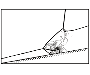
As shown in figure 1, a wedge of angle $\theta _{w}$ is immersed in an initially steady supersonic flow with Mach number $M_{0}$ and produces a steady oblique shock wave (AQ) with shock angle $\beta _{w}$. The incident shock is an oblique RMS which moves at a constant speed $u_{s}$ (in the normal direction). We use $p$, $\rho$, $T$, $a$, $M$ and $\theta$ to denote pressure, density, temperature, sound speed, Mach number and flow direction angle. We use $\gamma$ to denote the adiabatic index. We use subscripts $(l)$ and $(r)$ to denote variables in the left and right statuses of the RMOS. The shock wave moving Mach number is defined as $M_{s}=u_{s}/a_{r}$. In this paper we only consider the case that $M_{l}>1$, i.e. the inlet remains supersonic after the influence of the RMOS. The angle between the RMS and the horizontal direction is denoted as $\lambda$. Note that the angle $\lambda$ is not the shock angle. On the right of the RMOS the flow is horizontal, so $\theta _{r}=0$. The situation considered by Wang & Wu (2022) corresponds to $\lambda =90^{\circ }$ (and $\theta _{l}=0$).

Figure 1. Initial state of the reflection between an oblique RMS and a steady oblique shock wave attached to a sharp wedge (a) with $\lambda <90^{\circ },$ (b) with $\lambda >90^{\circ }$.

During reflection, the incident shock interacts with the oblique shock wave, as shown in figure 1(a) for $\lambda <90^{\circ }$ and figure 1(b) for $\lambda >90^{\circ }$.

Let ${\rm P}$ be the nominal intersection point between the RMS and the steady oblique shock wave. As shown in figure 2(a,b), the part of the RMS above the intersection point ${\rm P}$ will be denoted as $I_{S}$, meaning an incident shock wave. The pre-interaction part of the oblique shock is the unperturbed part $S_{OR}$. The post-interaction part is the perturbed steady oblique shock $S_{NE}$, which is the oblique shock wave newly created with a new inflow condition of region ($l$). Thus, point ${\rm P}$ is also the nominal intersection point of $I_{S}$ and $S_{OR}$. The nominal intersection point of $I_{S}$ and $S_{NE}$ is denoted ${\rm P}^{\prime }$.

Figure 2. Reflection between a right-going incident shock wave and a steady oblique shock wave attached to a sharp wedge (a) with $\lambda <90^{\circ },$ (b) with $\lambda >90^{\circ }$.

In the study of transition conditions, we need the flow parameters in regions ($l$), ($r$), ($d$) and ($dl$). Region (d) is downstream of the unperturbed shock $S_{OR}$ (see figure 1) and region $(dl)$ is downstream of the perturbed part $S_{NE}$ of the oblique shock wave. The flow parameters in region (r) will be given as input. The flow parameters in region ($l$) will be given in § 2.2.

The flow parameters in region (d) are connected to those in region $(r)$ through the following oblique shock wave relations:

(2.1)\begin{equation} \left. \begin{gathered} \tan\theta_{w}=f_{\theta}({M}_{r}{,\beta}_{w}),\\ M_{d}^{2}={f_{M}}(M_{r},\beta_{w}),\\ \frac{p_{d}}{p_{r}}={f_{p}}(M_{r},\beta_{w}),\\ \frac{\rho_{d}}{\rho_{r}}={f_{\rho}}(M_{r},\beta_{w}), \end{gathered} \right\} \end{equation}

where

(2.2) \begin{equation} \left. \begin{gathered} f_{\theta}({M,\beta})=\frac{2\left( {M}^{2}{\sin}^{2}{\beta}-1\right) } {[{M}^{2}(\gamma+\cos{2\beta)}+2]\tan{\beta}},\\ {f_{M}}(M,\beta)=\frac{{{M^{2}}+\dfrac{2}{{\gamma-1}}}}{{\dfrac{{2\gamma} }{{\gamma-1}}{M^{2}}{{\sin}^{2}}\beta-1}}+\frac{{{M^{2}}{{\cos}^{2}}\beta} }{{\dfrac{{\gamma-1}}{2}{M^{2}}{{\sin}^{2}}\beta+1}},\\ {f_{p}}(M,\beta)=1+\frac{{2\gamma}}{{\gamma+1}}[ {{{(M\sin\beta)}^{2} }-1}] ,\\ {f_{\rho}}(M,\beta)=\frac{{(\gamma+1){{(M\sin\beta)}^{2}}}}{{2+(\gamma -1){{(M\sin\beta)}^{2}}}} \end{gathered} \right\}. \end{equation}

The flow parameters in region $(dl)$ can be obtained using similar relations to the above, but with the upstream conditions replaced by those of region ($l$); more details will be given in § 4.

2.2. Method to give initial conditions

In order to consider the influence of $\lambda$, we determine the flow parameters in region $(l)$ from those in region $(r)$. The Mach number $M_{r}$ and the shock speed $u_{s}$ are the other two input parameters as considered before by Wang & Wu (2022).

Now let the flow parameters in region $(r)$ be given, and we provide below the expressions to determine the conditions in region $(l)$ for given shock speed $u_{s}$ and angle $\lambda$.

We use the subscript $n$ and $\tau$ to denote flow parameters normal to and tangent to the RMS and write $u_{r,n}=u_{r}\sin \lambda$, $u_{r,\tau }=u_{r} \cos \lambda$, $M_{r,n}=M_{r}\sin \lambda$, $M_{r,\tau }=M_{r}\cos \lambda$. The flow velocity component parallel to the RMS satisfies $u_{l,\tau }=u_{r,\tau }.$ According to Ben-Dor, Igra & Elperin (2000), for a moving shock of the first family we have

(2.3)\begin{equation} u_{s}=u_{r,n}-a_{r}\sqrt{\frac{\gamma+1}{2\gamma}\frac{p_{l}}{p_{r}} +\frac{\gamma-1}{2\gamma}}, \end{equation}

and

(2.4)\begin{equation} {u_{l,n}}={u_{r,n}}-\frac{{{a_{r}}}}{\gamma}\left( {\frac{{{p_{l}}}}{{{p_{r} }}}-1}\right) {\left( {\frac{{\gamma+1}}{{2\gamma}}\frac{{{p_{l}}}}{{{p_{r} }}}+\frac{{\gamma-1}}{{2\gamma}}}\right) ^{-{1}/{2}}}. \end{equation}

As usual, the speed of the incident shock can be measured with the shock moving Mach number defined as $M_{s}=u_{s}/a_{r}$, where $a_{r}$ is the sound speed in region $(r)$.

We use (2.3) to express the pressure ratio as a function of the Mach number $M_{r,n}$ and $M_{s}$

(2.5)\begin{equation} \frac{{{p_{l}}}}{{{p_{r}}}}=\psi(M_{r,n},M_{s}), \end{equation}

where

(2.6)\begin{equation} \psi(M_{r,n},M_{s})=\frac{2\gamma(M_{r,n}-M_{s})^{2}-(\gamma-1)}{\gamma+1}. \end{equation}

We then use the shock relation for density and the sound speed expression to write

(2.7a,b)\begin{equation} \frac{\rho_{l}}{\rho_{{{_{r}}}}}=\frac{{1+\dfrac{{\gamma+1}}{{\gamma-1}}}\psi }{\psi{\,+\,\dfrac{{\gamma+1}}{{\gamma-1}}}},\quad \frac{a_{l}}{a_{r}}=\sqrt {\psi\frac{\psi{\,+\,\dfrac{{\gamma+1}}{{\gamma-1}}}}{{1+\dfrac{{\gamma+1}} {{\gamma-1}}}\psi}}. \end{equation}

Insert (2.4) for $u_{l,n}$ and (2.7a,b) for $a_{l}$ into ${M_{l,n}}=u_{l,n}/a_{l}$, and use (2.5) to replace $p_{l}/p_{r}$ by $\psi$, we get, for the RMS of the first family

(2.8)\begin{equation} {M_{l,n}}=\frac{{M_{r,n}}-\dfrac{{1}}{\gamma}\left( \psi{-1}\right) {\left( {\dfrac{{\gamma+1}}{{2\gamma}}\psi+\dfrac{{\gamma-1}}{{2\gamma}}}\right) ^{-{1}/{2}}}}{\sqrt{\psi\dfrac{\psi{\,+\,\dfrac{{\gamma+1}}{{\gamma-1}}} }{{1+\dfrac{{\gamma+1}}{{\gamma-1}}}\psi}}}. \end{equation}

In summary, with $M_{r},u_{r},\rho _{r},p_{r}$ on the right of the RMS and the shock speed $u_{s}$ given, we use (2.5), (2.6) and (2.7a,b) to obtain $p_{l},\rho _{l},a_{l}$. Then, we use (2.4) and $u_{l,\tau }=u_{r,\tau }$ to obtain $u_{l,n}$ and $u_{l,\tau }$. The shock angle $\beta _{lr}$ of the RMS can be derived from $\beta _{lr}=\arctan ({u_{l,n} /}u_{l,\tau })$. After that, the flow direction $\theta _{l}$ in region ($l$) can be derived from

(2.9)\begin{equation} \left. \begin{array}{@{}ll@{}} \theta_{l}=\beta_{lr}+\lambda-180^{{\circ}}, & \text{if }\lambda>90^{{\circ}},\\ \theta_{l}=\lambda-\beta_{lr}, & \text{if }\lambda<90^{{\circ}}. \end{array} \right\} \end{equation}

See figure 3 for notations. The velocity components $(u_{l},v_{l})$ in region ($l$) can finally be derived from

(2.10a,b)\begin{equation} u_{l}=\sqrt{{u_{l,n}^{2}}+u_{l,\tau}^{2}}\cos\theta_{l},\quad v_{l}=\sqrt {{u_{l,n}^{2}}+u_{l,\tau}^{2}}\sin\theta_{l} . \end{equation}

Figure 3. Schematic illustration of the relation between $\theta _{l}$, $\beta _{lr}$ and $\lambda$; (a) $\lambda >90^{\circ }$, (b) $\lambda <90^{\circ }$.

2.3. Method for numerical simulation

For numerical simulation, the compressible Euler equations of an ideal gas are solved using the second-order advection upstream splitting method (Liou 1996). The computational domain and boundary conditions are displayed in figure 4(a). The flow field around a wedge with a wedge angle $\theta _{w}$ is simulated. The lower and upper boundaries are designed as the supersonic inlet boundary, for which the deflection angle $\theta _{1}$ and $\theta _{2}$ satisfies $\theta _{1}>-\theta _{l}$ and $\theta _{2}>\theta _{l}$ to ensure fluid flow into the computational zone.

Figure 4. (a) Computational domain and boundary conditions. (b) Number of grids along two directions, with three blocks of structured mesh separated with dashed lines.

As in Wang & Wu (2022), the computation is performed with two steps. First, the steady solution without the RMS is calculated. Then, the RMS is imposed and the unsteady flow field is calculated within the second step. To impose the RMS, we need to initialize the flow field in region ($l$), using the method provided in § 2.2, and set the boundary condition in the supersonic inlet boundaries into a timely changing condition with the upstream and downstream flow parameters of the RMS.

Once the interaction takes place, the problem enters into a pseudo-steady state which has no characteristic scales so that the flow field is self-similar. Hornung (1986) gives a review of shock reflection, stating that the introduction of any length scale independent of the travelling distance will break the self-similarity. Pseudo-steady solution has been studied in a number of problems with shock waves. Jones et al. (1951) showed the existence of self-similar flow behind a strong shock diffracting or reflecting at a corner. They transformed the equations of an unsteady compressible flow for a pseudo-stationary problem into a steady compressible flow problem with non-conservative field of external forces and sinks. Shock diffraction at a convex corner and regular reflection beyond a concave corner is also considered. Tesdall, Sanders & Keyfitz (2008) presented numerical solutions for a self-similar solution for weak Mach reflection. Martínez-Ruiz et al. (2019) considered the impingement of a shock wave on shear layers, and discussed the self-similar regime of this problem. In § 5, the self-similar nature of the flow will be discussed.

According to Jones et al. (1951), a flow is pseudo-stationary about the origin of coordinates if, in terms of the new coordinates $\xi =x/t$, $\eta =y/t$, $\zeta =t$, it is independent of $\zeta$. Thus, we only need to output the flow field at same typical instant that is short enough to avoid unnecessary calculation and is long enough for the flow details to be visible.

To see the sensitivity of the results to the grid resolution, we choose $M_{r}=6$, ${M_{S}=5.5}$, $\theta _{w}=10^{\circ }$ and $\lambda =83^{\circ }$, and use three grids defined in table 1. The mesh density in the computational domain is illustrated in figure 4(b). The Mach contours at the same typical instant are displayed in figure 5. The results of grid 3 have little difference from the results of grid 2. Hence, we will use mesh density similar to grid 2 for all the numerical simulations in this paper.

Table 1. Three grids tested. Here, $n_{x}$ represents the number of mesh cells along the $x$ direction along the wedge surface and $n_{y}$ represents the number of mesh cells in the perpendicular direction.

Figure 5. Comparison of Mach contour for (a) mesh 1, (b) mesh 2 and (c) mesh 3 in table 1.

2.4. Observation of pre-shock reflection and post-shock reflection

Here, we use two typical cases to demonstrate pre-shock reflection and post-shock reflection, as mentioned in the Introduction.

The first case has ${M_{r}=6},$ ${M_{S}=5.5}$, ${\theta _{w}=10}$ and $\lambda =85^{\circ }$. The Mach contours in the fixed frame (also called ground frame) are shown in figure 6(a,b). Figure 6(a,b) displays in addition streamlines, using velocities in the frame co-moving with the nominal intersection point ${\rm P}$ and ${\rm P}^{\prime }$, respectively, see figure 6(c) for a sketch of the configuration(with slip lines represented by double parallel lines). From the streamlines shown in figure 6(a) we see pre-shock reflection, that is, the incident shock ($I_{S}$) reflects over the pre-interaction part ($S_{OR}$) of the steady oblique shock wave. Moreover, this pre-shock reflection is equivalent to the problem of shock interaction between two shock waves from the same side.

Figure 6. Numerical results for case pre-IV-1 in table 2 ($M_{r}=6,$ ${M_{S}=5.5}$, $\theta _{w}=10$ and $\lambda =85^{\circ }$), (a) Mach contours in the fixed frame and streamlines in the co-moving frame of P, (b) Mach contours in the fixed frame and streamlines in the co-moving frame of ${\rm P}^{\prime }$, (c) sketch of shock structures and nominal intersection points ${\rm P}$ and ${\rm P}^{\prime }$.

The second case has $M_{r}=6,$ $M_{S}=2.4$, $\theta _{w}=10$ and $\lambda =149^{\circ }$. The Mach contours in the fixed frame are shown in figure 7(a). Figure 7(a) displays in addition streamlines, using velocities in the frame co-moving with the nominal intersection point ${\rm P}^{\prime }$. See figure 7(b) for a sketch of the configuration. It is seen from the streamlines shown in figure 7(a) that post-shock reflection as defined in the Introduction happens. Moreover, this post-shock reflection is a shock interaction between two shock waves ($I_{S}$ and $S_{NE}$) from opposite sides.

Figure 7. Numerical results for case post-I-1 in table 2 ($M_{r}=6,$ $M_{S}=2.4$, $\theta _{w}=10$ and $\lambda =149^{\circ }$). (a) Mach contours in the fixed frame and streamlines in the co-moving frame of ${\rm P}^{\prime }$, (b) sketch of shock structures and nominal intersection point ${\rm P}^{\prime }$.

In summary, pre-shock reflection is the interaction between the incident shock $I_{S}$ and the pre-interaction shock $S_{OR}$ (and below we will use the prefix pre- to denote such reflection types), post-shock reflection is the interaction between the incident shock $I_{S}$ and the post-interaction shock $S_{NE}$ (and below we will use the prefix post- to denote such reflection types). Pre-shock reflection and post-shock reflection will be studied in §§ 3 and 4, respectively. In § 5, we will discuss which situations occur in a specific region.

In § 5, we will consider more cases to verify the transition conditions given in §§ 3 and 4, and to study more detailed flow structures. These test cases are summarized in table 2.

Table 2. Nine test cases.

2.5. Edney's six types of shock interaction

As stated above, the pre-shock reflection is equivalent to the problem of shock interaction between two shock waves from the same side, the post-shock reflection is a shock interaction between two shock waves from opposite sides. These situations occur in the six types of shock interference (Edney 1968), as illustrated in figure 8, where an incident shock wave interacts with a detached bow shock of a blunt body.

Figure 8. Edney's six types of shock interaction.

When the incident shock wave intersects the lower part of the bow shock, the incident shock and the bow shock before the nominal intersection point are from opposite sides, which may lead to three types of shock interference known as type I, type II and type III shock interferences. Type I and II shock interferences occur when the incident shock intersects the bow shock at its weak part, which may produce regular reflection (type I shock interference) or irregular reflection (type II shock interference). If the incident shock intersects the bow shock at its strong part (before the sonic line $M=1$ as shown in figure 8), we have type III shock interference which has two triple points ($A$ and $B$). When the incident shock wave intersects the upper part of the bow shock, the incident shock and the bow shock before the nominal intersection point are from the same side, which may lead to three types of shock interferences known as type IV, type V and type VI shock interferences. Type V and VI shock interferences occur when the incident shock intersects the bow shock at its weak part, which may produce regular reflection (type VI shock interference) or irregular reflection (type V shock interference, which has three triple points). If the incident shock intersects the bow shock at its strong part (before the sonic line $M=1$ as shown in figure 8), we have type IV shock interference (which has two triple points, similar to type III shock interference).

Type VI also needs to be mentioned, since it contains two subcases. The reflected wave AB is either an expansion fan (usual type VI shock interference) or a compression wave (called type VI-I shock interference).

Edney (1968) has described the details of each type of shock interference. Each shock interference can be analysed using the knowledge from shock reflection. Consider, for instance, type IV shock interference. The incident shock (IS) intersects the bow shock to create a triple point (A), like the triple point observed in Mach reflection. Here, the triple point A connects the IS, a Mach stem (AA$^{\prime }$, which is the unperturbed bow shock), a reflected shock (AB) and a slipline (AC). The reflected shock AB then intersects the lower part of the bow shock to create the second tripe point (B), which connects the shock AB, a Mach stem (BB$^{\prime }$, which is the lower part of the bow shock), a reflected shock (BC) and a slipline. The reflected shock BC then reflects between the two sliplines to create a supersonic jet.

The six types of shock interferences produced by the impingement of an IS on a bow shock (as shown in figure 8) has been well studied in the past. Apart from the work of Edney (1968) who identified the six types of shock interference using experiments and theoretical analyses, Bramlette (1974) described an approximate method to compute type III and type IV shock interferences and predict the transition condition between them. Keyes & Hains (1973) theoretically and experimentally analysed the aerodynamic heating of six types of shock interference.

3. Study of transition condition for pre-shock reflection

In this section we study pre-shock reflection considering $\lambda$, with $0^{\circ }<\lambda <180^{\circ }$. The study of Wang & Wu (2022) only considers $\lambda =90^{\circ }$.

3.1. Method for transition condition on the equivalent problem

The reflection types and transition conditions are studied by using the equivalent steady-state problem, defined in the frame attached to the nominal intersection point P (see figure 9). Pre-shock reflection is the reflection where the shock waves $I_{S}$ and $S_{OR}$ are assumed to be incident shocks. For the equivalent steady-state problem, we further assume that $I_{S}$ and $S_{OR}$ are from the same side, so we expect to have three types of reflection, called pre-IV, pre-V and pre-VI reflections, in connection with the classical type IV, type V and type VI shock interferences (presented in § 2.5). For each of this anticipated reflection configuration, we perform numerical simulation using a typical flow condition, and a switch between the numerical results and the classical shock interference types can be done using frame transformation as described below.

Figure 9. Flow parameters in the frame co-moving with the nominal intersection point P.

In the study for $\lambda =90^{\circ }$, Wang & Wu (2022) made a switch of one type of shock on shock interaction to type V shock interference (see figure 11 of Wang & Wu 2022). This switch is done as follows in more general cases. Draw the streamlines and Mach contour lines of the flow field obtained from numerical simulation using the data in the frame co-moving with the measured nominal intersection point (P), then flip upside down and rotate the picture until the flow configuration is comparable to one of the flow patterns as displayed in figure 8. In this way we can identify three flow patterns, as shown in figure 10. Pre-IV corresponds to the classical type IV shock interference as shown in figure 8. Similarly, pre-V corresponds to the classical type V shock interference and pre-VI corresponds to the classical type VI shock interference.

Figure 10. Illustration of possible shock patterns for the situation that $I_{S}$ interacts with $S_{OR}$.

The method to analyse the critical conditions for six types of shock interference (cf. Crawford 1973; Bramlette 1974; Olejniczak, Wright & Candler 1997; Grasso et al. 2003) can then be applied to the equivalent problem of the pre-shock reflection to obtain the critical conditions of pre- IV, pre-V and pre- VI shock interferences, in a similar way as Wang & Wu (2022).

Now it remains to obtain the flow conditions of the equivalent problem needed to analyse the transition conditions. First, we need the velocity $\boldsymbol {V_{P}}$ of the nominal intersection point P. The expression of this velocity is easily found to be $\boldsymbol {V_{P}}=(u_{P},v_{P})$ where

(3.1a,b)\begin{equation} u_{p}=\frac{M_{s}a_{r}}{\sin(\lambda-\beta_{w})}\cos\beta_{w},\quad v_{p} =\frac{M_{s}a_{r}}{\sin(\lambda-\beta_{w})}\sin\beta_{w}, \end{equation}

where $\beta _{w}$ is the shock angle provided by (2.1).

At a reference frame attached to P, the flow velocities in various regions shown in figure 9 are

(3.2)\begin{equation} \left. \begin{gathered} (u_{r}^{(P)},v_{r}^{(P)})=(u_{r}-u_{P},-v_{P})\text{ region }(r),\\ (u_{l}^{(P)},v_{l}^{(P)})=(u_{l}-u_{P},v_{l}-v_{P})\text{ region }(l),\\ (u_{d}^{(P)},v_{d}^{(P)})=(u_{d}-u_{P},v_{d}-v_{P})\text{ region }(d), \end{gathered} \right\} \end{equation}

where $u_{P}$ and $v_{P}$ are given by (3.1a,b).

The input parameters for the equivalent steady problem are given as $M_{0}=M_{l}^{(P)}$, $M_{1}=M_{r}^{(P)}$, $M_{2}=M_{d}^{(P)}$, $\theta _{1}=\theta _{r}^{(P)}-\theta _{l}^{(P)},$ $\theta _{2}=\theta _{d}^{(P)} -\theta _{l}^{(P)}$, where the Mach numbers $M_{l}^{(P)}$, $M_{r}^{(P)}$, $M_{d}^{(P)}$ and the flow deflection angles $\theta _{l}^{(P)}$ , $\theta _{r}^{(P)}$, $\theta _{d}^{(P)}$ are computed using the velocities defined by (3.2). The flow deflection angle $\Delta \theta$ of the second attached shock wave of the equivalent double wedge shock reflection problem satisfied $\Delta \theta =\theta _{1}-\theta _{2}$.

For pre-shock reflection study we only consider reflection at the nominal intersection point ${\rm P}$ and the perturbation from post-shock reflection at the other nominal intersection point is omitted. As such, the incident shocks $I_S$ and $S_{OR}$ are assumed to be straight.

3.2. Transition conditions for pre-shock reflection

We present transition conditions in the $M_{s}-\lambda$ plane for $M_{r}=6$ and for four values of $\theta _{w}$ ($\theta _{w}=5^{\circ }$, $10^{\circ }$, $15^{\circ }$, $20^{\circ }$). The range for $M_{s}$ is determined from the requirement that the incident shock wave ($I_{S}$) is of the first family. The results are given in figure 11. Five regions, labelled pre-DAR, pre-IV, pre-V, pre-VI-I and pre-VI, are identified.

Figure 11. Regions having different shock patterns for interaction between incident shock and unperturbed shock in $M_{s}-\lambda$ plane for $M_{r}=6$, (a) with $\theta _{w}=5^{\circ }$, (b) with $\theta _{w}=10^{\circ }$, (c) with $\theta _{w}=15^{\circ }$, (d) with $\theta _{w}=20^{\circ }$.

The five regions are bounded between a left boundary and a right boundary (as marked in figure 11a). Now we give the expressions for these boundaries. Since the shock $I_{S}$ is of the first family we have $0<\psi ={{{p_{l}}}}/{{{p_{r}}}}\leq 1$, and, by (2.6),

(3.3)\begin{equation} M_{r}\sin\lambda-\sqrt{\frac{\gamma-1}{2\gamma}}>M_{S}>M_{r}\sin\lambda-1. \end{equation}

Thus, the left and right boundaries of the five regions are defined by $M_{S}=M_{r}\sin \lambda -1$ and $M_{S}=M_{r}\sin \lambda -\sqrt {({\gamma -1})/{2\gamma }}$, respectively.

The three regions labelled pre-IV, pre-V and pre-VI in figure 11 correspond to type IV, type V and type VI shock interferences as shown in figure 10. There is a subregion labelled pre-VI-I, corresponding to type VI-I shock interference, as pointed out in § 2.5.

Shock polars are given in figure 12, for the typical cases shown in table 2, which are also labelled with pre-IV-1, pre-V-1, pre-VI-1, pre-VI-2 and marked with red circles and red text in figure 11(b). Shock polars are obtained for the equivalent problem for all cases. Polar $\varGamma _{i}$ stands for the shock with upstream region (i). For instance, polar $\varGamma _{0}$ stands for the shock with upstream parameters specified. The intersection of two polars means the downstream of the two shocks reaches an equilibrium of the mechanical problem, including the flow deflection angle and pressure. Consider, for instance, figure 12(a) for a shock polar of pre-IV, the intersection point of polar $\varGamma _{0}$ and $\varGamma _{1}$ gives an equilibrium state between regions ($2$) and $(3)$, i.e. for the first triple point, the flow in regions (2) and (3) is parallel near the slipline, and the pressure in regions (2) and (3) is balanced near the slipline. The same holds true for the second triple point, which connects the shock between regions (1) and (3), the shock between regions (1) and (5) and the shock between regions (3) and (4). The shock polar for pre-V displayed in figure 12(b) shows why a third triple point appears and this triple point, downstream of which we have regions $(7)$ and $(8)$, which is the intersection point of polars $\varGamma _{1}$ and $\varGamma _{6}$. The shock polars displayed in figure 12(c,d) are for the two subcases of pre-VI, one has a compression reflected wave and the other has an expansion reflected wave.

Figure 12. Shock polars in the co-moving frame of ${\rm P}$ for pre-interaction for cases marked in figure 11(b).(a) Pre-IV-1. (b) Pre-V-1. (c) Pre-VI-1. (d) Pre-VI-2.

Region pre-DAR means no solution. In fact, in this region, had we assumed pre-shock reflection occurs, we would have deflection angle reversal, as observed in Wang & Wu (2022) for $\lambda =90^{\circ }$. Flow deflection reversal means that the flow deflection across $S_{OR}$ becomes negative so $S_{OR}$ is no longer an incident shock but a reflected shock. In conclusion, region pre-DAR is impossible for pre-shock reflection to occur and may just allow for post-shock reflection, to be considered in § 4.

Curve AB is the transition condition from impossible pre-shock reflection (pre-DAR) to type IV shock interference. Curve CD is the transition condition between type ${\rm IV}$ and type ${\rm V}$ shock interference. Curve EF is the transition condition between type ${\rm V}$ and type ${\rm VI}$ or ${\rm VI}-{\rm I}$ shock interference.

It is seen that type VI shock interference occurs for small $\lambda$. Increasing $\theta _{w}$ increases the regions for type IV, type V and type VI shock interferences.

The transition conditions can also be viewed in the $\theta _{w}-\lambda$ plane. For $M_{r}=6$ and for three values of $M_{s}$ ($M_{S}=3,$ $4,$ $5.3$), the conditions are displayed in figure 13. The range for $\lambda$ is still determined from the requirement that the incident shock wave is of the first family.

Figure 13. Regions having different shock reflection patterns in $\theta _{w}-\lambda$ plane for $M_{r}=6$, (a,b) with $M_{S}=3,$ (c) with $M_{S}=4,$ (d) with $M_{S}=5.3$.

Since figure 13 is just another view of figure 11, we just point out the possible new features revealed in this new plane.

For $M_{S}=3$, for which the results are displayed in figure 13(a), we have two disconnected regions: one for large $\lambda$, where we may have pre-DAR and pre-IV, the other for small $\lambda$, where we may have pre-IV, pre-V and pre-VI. Figure 13(b) shows an enlarged view of the region with various reflection types. The reason to have two disconnected regions can be understood from what has been shown in figure 11: a vertical line at a given $M_{S}$ should intersect the entire region at two disconnected parts, which, when $\theta _{W}$ spans a finite interval, form the two disconnected regions, as shown in figure 13(a).

Figure 13(c) displays the results for $M_{S}=4$, and similarly as the case with $M_{S}=3$, we have two disconnected regions, the difference is that the two disconnected regions get closer (the reason can be seen from the curve shapes of the two boundaries displayed in figure 11).

For $M_{S}=5.3$, for which the results are displayed in figure 13(d), we only have one region for shock reflection, that lies between $\lambda =75^{\circ }$ and $110^{\circ }$. First, by figure 11, it is clear that, for large $M_{S}$, a vertical line cuts only one region so we have only one region for shock reflection. Second, the condition for one region can be derived. Now we derive the critical condition $M_{S}=M_{S}^{(cri)}$ beyond which we have only one connected region.

According to figure 11, if $M_{S}$ on the right of the left boundary $M_{S}=M_{r}\sin \lambda -1$, then we have only one connected region. Thus, the critical value $M_{S}^{(cri)}$ corresponds to the right most point of $M_{S}=M_{r}\sin \lambda -1$, i.e.

(3.4)\begin{equation} M_{S}^{(cri)}=M_{r}-1. \end{equation}

Thus, with $M_{S}>M_{r}-1$, there is only one simple connected region and with $M_{S}< M_{r}-1$, there is a doubly connected region.

4. Study of transition condition for post-shock reflection

In this section, we study post-shock reflection considering $\lambda$, with $0^{\circ }<\lambda <180^{\circ }$. Again the study of Wang & Wu (2022) only considers $\lambda =90^{\circ }$.

4.1. Method for transition condition on the equivalent problem

The reflection types and transition conditions are studied by using the equivalent steady problem, defined in the frame attached to the nominal intersection point ${\rm P}^{\prime }$. Figure 14(a) illustrates the problem in the ground frame, and figure 14(b) in the frame comoving with ${\rm P}^{\prime }$. Post-shock interaction is the reflection where the shock waves $I_{S}$ and $S_{NE}$ are assumed to be incident shock waves. The two incident shocks $I_{S}$ and $S_{NE}$ are from opposite sides, so for the equivalent problem, we are expected to have three types of post-shock reflection, corresponding to the type I, type II and type III shock interferences presented in § 2.5.

Figure 14. Schematic illustration of shock angle $\beta _{1}^{(P^{prime})}$ and $\beta _{2}^{(P^{prime})}$ in the co-moving frame of intersection point P$^{\prime }$. (a) Flow in the co-moving frame with A. (b) Flow in the co-moving frame with P$^{\prime }$.

For each of these anticipated reflection configurations, we perform numerical simulation using a typical flow condition, and a switch between the numerical results and the classical shock interference types can be done using the switch method as described in § 3.1. In this way we can identify the possible flow patterns.

Type III shock interference is slightly more complicated here. We do not find type III shock interferences for the present problem. However, in the frame co-moving with point ${\rm P}^{\prime }$, there are conditions for which either $I_{S}$ or $S_{NE}$ becomes a strong shock wave. In the classical six types of shock interference of Edney, we normally have type III shock interference as shown in figure 8. But in the usual type III shock interference, there is only one incident shock, and here both $I_{S}$ and $S_{NE}$ play the role of incident shock waves as in asymmetric shock reflection, so we still have type II shock interference. To distinguish this from the usual type II shock interference, we use post-IIa to denote that shock reflection type when $I_{S}$ is strong in the frame co-moving with point ${\rm P}^{\prime }$ and post-IIb when $S_{NE}$ in the frame co-moving with point ${\rm P}^{\prime }$ is a strong shock wave.

Figure 15 displays post-I and post-II shock reflections, which are obviously similar to type I and type II shock interferences.

Figure 15. Illustration of possible shock patterns for the situation that $I_{S}$ interacts with $S_{NE}$.

Post-I and post-II in the frame co-moving with point ${\rm P}^{\prime }$ define in fact asymmetric shock reflection. The transition conditions for these two types of post-shock reflection can then be decided using the traditional asymmetric shock reflection transition conditions proposed in Li, Chpoun & Ben-Dor (1999), with the input parameters $M_{l}^{(P^{\prime })}$, $\beta _{1}^{(P^{\prime })}$ and $\beta _{2}^{(P^{\prime })}$ (see figure 14b) given. The regions to have regular and Mach reflection correspond to post-I and post-II reflections, separately. The detachment condition and the von Neumann condition may hold a common region called the double solution region and is denoted post-DSD below. We find that, in the frame co-moving with point ${\rm P}^{\prime }$, one of the shock wave $I_{S}$ or $S_{NE}$ may become a strong shock wave.

Now it remains to obtain the flow conditions for the equivalent problem needed to analyse the transition conditions. The flow parameters for the original problem and equivalent problem have been displayed separately in figure 14(a,b). First, we need the velocity $\boldsymbol {{V}_{P^{\prime }}}$ of point ${\rm P}^{\prime }$. The expression of this velocity is easily found to be ${\boldsymbol {{V}_{P^{\prime }}}=(u_{P^{\prime } },v_{P^{\prime }})}$ where

(4.1a,b)\begin{equation} u_{P^{\prime}}=\frac{M_{s}a_{r}}{\sin(\lambda-\beta_{NE})}\cos\beta_{NE},\quad v_{P^{\prime}}=\frac{M_{s}a_{r}}{\sin(\lambda-\beta_{NE})}\sin\beta_{NE}, \end{equation}

where $\beta _{NE}$ is the angle between the newly formed oblique shock wave $S_{NE}$ and the horizontal line and is given by

(4.2)\begin{equation} \beta_{NE}=\bar{\beta}_{w}+\theta_{l}, \end{equation}

where $\bar {\beta }_{w}$ is the shock angle of $S_{NE}$ defined on the fixed frame and is determined by the shock angle relation $\tan \bar {\theta } _{w}=f_{\theta }(M_{l}{,}\bar {\beta }_{w})$ (see (2.2) for definition of $f_{\theta }(M{,}\beta )$) with $\bar {\theta }_{w}=-\theta _{l}+\theta _{w}$. Here, $\tan \bar {\theta }_{w}=f_{\theta }(M_{l}{,}\bar {\beta }_{w})$ is solved for the weak solution. In the co-moving frame, the flow velocity and Mach number in region ($l$) are thus

(4.3)\begin{equation} \left. \begin{gathered} (u_{l}^{(P^{\prime})},v_{l}^{(P^{\prime})})=(u_{l}-u_{P^{\prime}} ,v_{l}-v_{P^{\prime}}),\\ M_{l}^{(P^{\prime})}=\frac{\sqrt{\left( \left( u_{l}^{(P^{\prime})}\right) ^{2}+\left( v_{l}^{(P^{\prime})}\right) ^{2}\right) }}{a_{l}}, \end{gathered} \right\} \end{equation}

where $u_{P^{\prime }}$ and $v_{P^{\prime }}$ are defined by (4.1a,b). The flow direction angle $\theta _{l}^{(P^{\prime })}$ in the co-moving frame is given by

(4.4) \begin{equation} \left. \begin{array}{@{}ll@{}} \theta_{l}^{(P^{\prime})}=\arctan\left\vert \dfrac{v_{l}^{(P^{\prime})}} {u_{l}^{(P^{\prime})}}\right\vert, & \text{if }u_{l}^{(P^{\prime})} >0,v_{l}^{(P^{\prime})}>0,\\ \theta_{l}^{(P^{\prime})}={\rm \pi}-\arctan\left\vert \dfrac{v_{l}^{(P^{\prime})} }{u_{l}^{(P^{\prime})}}\right\vert, & \text{if }u_{l}^{(P^{\prime})} <0,v_{l}^{(P^{\prime})}>0,\\ \theta_{l}^{(P^{\prime})}={\rm \pi}+\arctan\left\vert \dfrac{v_{l}^{(P^{\prime})} }{u_{l}^{(P^{\prime})}}\right\vert , & \text{if }u_{l}^{(P^{\prime})} <0,v_{l}^{(P^{\prime})}<0,\\ \theta_{l}^{(P^{\prime})}=2{\rm \pi}-\arctan\left\vert \dfrac{v_{l}^{(P^{\prime})} }{u_{l}^{(P^{\prime})}}\right\vert , & \text{if }u_{l}^{(P^{\prime})} >0,v_{l}^{(P^{\prime})}<0. \end{array} \right\} \end{equation}

The shock angles $\beta _{1}^{(P^{\prime })}$ and $\beta _{2}^{(P^{\prime })}$ of the two incident shocks $I_{S}$ and $S_{NE}$, as shown in figure 14(b), are therefore given by

(4.5)\begin{equation} \left. \begin{gathered} \beta_{1}^{(P^{\prime})}={\rm \pi}-\lambda+\theta_{l}^{(P^{\prime})},\\ \beta_{2}^{(P^{\prime})}=\beta_{NE}-\theta_{l}^{(P^{\prime})}. \end{gathered} \right\} \end{equation}

For post-shock reflection study we only consider reflection at the nominal intersection point ${\rm P}^{\prime }$ and the perturbation from pre-shock reflection at the other nominal intersection point (${\rm P}$) is omitted. As such, the incident shocks $I_{S}$ and $S_{NE}$ are assumed to be straight.

4.2. Transition conditions for post-shock reflection

As for pre-shock reflection, we present transition conditions in the $M_{s}-\lambda$ plane for ${M_{r}=6}$ and for four values of $\theta _{w}$ ($\theta _{w}=5^{\circ }$, $10^{\circ },$ $15^{\circ }$, $20^{\circ }$). The range for $M_{s}$ is also determined from the requirement that the incident shock wave is of the first family. The results are given in figure 16, where we have five regions, labelled post-I, post-DSD, post-II, post-IIa, post-IIb. The left and right boundaries of these regions are still given by (3.3).

Figure 16. Regions to have different shock patterns for interaction between incident shock and perturbed shock in $M_{s}-\lambda$ plane for $M_{r}=6$, (a) with $\theta _{w}=5^{\circ }$, (b) with $\theta _{w}=10^{\circ }$, (c) with $\theta _{w}=15^{\circ }$, (d) with $\theta _{w}=20^{\circ }$.

The two regions labelled post-I and post-II in figure 16 correspond to type I and type II interferences, or regular and Mach reflections. The region marked post-DSD is the double solution domain, where we may have both regular and Mach reflections. As stated in § 4.1, the regions denoted post-IIa and post-IIb also belong to type II shock interference, but with one of the incident shocks being a strong one in the equivalent problem.

Shock polars are given in figure 17, for the typical cases shown in table 2, and labelled with post-I-1, post-I-2, post-II-1, post-II-2 and marked with red circles and red text in figure 16(b). As for pre-shock reflection, here, shock polars are obtained for the equivalent problem for all cases. See the description of figure 12 for more explanation. Figure 17(a) is the shock polar of post-I with a very large $\lambda$, the intersection point of polar $\varGamma _{1}$ and $\varGamma _{2}$ gives an equilibrium state between regions ($3$) and $(4)$, i.e. the flow in regions (3) and (4) is parallel near the slipline, and the pressure in regions (3) and (4) is balanced near the slipline. For a smaller $\lambda$, the shock polars are displayed in figure 17(b), from which we see that the pressure in region (3) or (4) is increased. This increase is due to the fact that reducing $\lambda$ will increase the shock angles defined by (4.5). Figure 17(c,d) shows shock polars for post-II, one for large $\lambda$ and one for small $\lambda$, showing the mechanism to have two triple points, and showing how $\lambda$ affects the equilibrium pressure through changing the shock angles defined by (4.5).

Figure 17. Shock polars in the co-moving frame of ${\rm P}^{\prime }$ for post-interaction for cases marked in figure 16(b). (a) Post-I-1. (b) Post-I-2. (c) Post-II-1. (d) Post-II-2.

We observe that regular reflection (post-I) occurs for large $\lambda$ and Mach reflection (post-II) occurs for large $M_{s}$. The reason is that, when $\lambda$ is large, the two incident shocks $I_{S}$ and $S_{NE}$ intersect at an angle small enough to have smaller shock angles $\beta _{1}^{(P^{\prime })}$ and $\beta _{2}^{(P^{\prime })}$ as described by (4.5), so that regular reflection is favoured. For large $M_{s}$, it can be verified that the upstream Mach number $M_{l}^{(P^{\prime })}$ defined by (4.3) is reduced, so as in asymmetric shock reflection, Mach reflection, is favoured.

We also observe that the region with double solution (post-DSD) varies with $\theta _{w}$, and for $\theta _{w}=5^{\circ }$, this region almost vanishes. This can also be understood from the critical conditions of the corresponding equivalent asymmetric reflection, where the region for a double solution reduces when one of the angles becomes small (see figure 7 of Li et al. 1999).

Moreover, we observe that the region for Mach reflection has a complex shape, type post-IIa reflection occurs only for small $\theta _{w}$, i.e. for $\theta _{w}=5^{\circ }$, and type post-IIb reflection occurs for small $\lambda$, and the region with this reflection increases for larger $\theta _{w}$. These observations can be understood by considering how the flow parameters change the transition conditions on the equivalent asymmetric reflection, in a similar way as above.

The transition conditions can also be displayed in the $\theta _{w}-\lambda$ plane. For $M_{r}=6$ and for three values of $M_{s}$ ($M_{S}=3,$ $4,$ $5.3$) the results are displayed in figure 18. Similarly to pre-shock reflection, for which similar results are presented in figure 13, we also have two disconnected regions.

Figure 18. Regions having different shock reflection patterns in $\theta _{w}-\lambda$ plane for $M_{r}=6$, (a) with $M_{S}=3,$ (b) with $M_{S}=4,$ (c) with $M_{S}=5.3$.

For $M_{S}=3$, for which the results are displayed in figure 18(a), we have two disconnected regions: one for large $\lambda$ where we may have post-DSD and post-II, the other for small $\lambda$, where we may have post-IIa and post-IIb. The reason for having two disconnected regions can be understood from what has been shown in figure 16: a vertical line at a given $M_{S}$ should intersect the entire region at two disconnected parts, which, when $\theta _{W}$ spans a finite interval, form the two disconnected regions as shown in figure 18(a).

For $M_{S}=4$, for which the results are displayed in figure 18(b), the situation is similar to case with $M_{S} =3$, except the two regions get closer. The reason can be seen from the curve shapes of the two boundaries displayed in figure 16.

For $M_{S}=5.3$, for which the results are displayed in figure 18(c), we only have one region of shock reflection, that lies between $\lambda =70^{\circ }$ and $110^{\circ }$. The critical condition $M_{S}=M_{S}^{(cri)}$ beyond which we have only one connected region is similar to that discussed for pre-shock reflection, i.e. $M_{S}^{(cri)}$ is given by (3.4).

5. Numerical simulation and classification

In this section, we use numerical simulation for the test cases shown in table 2 to clarify how the predicted pre-shock reflection and post-shock reflection, which would appear at the two different nominal intersection points ${\rm P}$ and ${\rm P}^{\prime }$, exist alone or coexist in the full flow configuration.

5.1. Possibility of combination of pre- and post-shock reflections

The transition study presented in § 3 for pre-shock reflection only predicts the possible reflection configuration at the nominal intersection point ${\rm P}$ and the transition study presented in § 4 for post-shock reflection only predicts the possible reflection configuration at the nominal intersection point ${\rm P}^{\prime }$ (see figure 2). In real situations, both nominal intersection points exist, so that reflection may occur at only one of these two points, or at both. According to figure 19(a,b), there are regions for which we may have post-shock reflection and no pre-shock reflection, or both, so we may have the following two possibilities.

Figure 19. Cases marked with integral number in regions having different shock reflection patterns in $M_{s}-\lambda$ plane for $M_{r}=6$ with $\theta _{w}=10^{\circ }$; (a) the reflection type around point ${\rm P}$ for the interaction of $I_{S}$ and $S_{OR}$, (b) the reflection type around point ${\rm P}^{\prime }$ for the interaction of $I_{S}$ and $S_{NE}$.

1. (i) post-shock reflection dominated, for which the post-shock reflection is as predicted by the theory of § 4 and pre-shock reflection does not exist theoretically (corresponding to the region pre-DAR in figure 19(a)) and, if it still exists, it should be a result of further interaction (due to a post-shock reflection produced shock interacting with the pre-interaction part of the oblique shock wave);

2. (ii) combined pre-shock reflection and post-shock reflection, both are predicted by theory (§§ 3 and 4, and as shown in figure 19).

Nine typical cases shown in table 2 and also marked in figure 19 as post-I-1, post-I-2, post-II-1, post-II-2, post-II-3, pre-IV-1, pre-V-1, pre-VI-1, pre-VI-2 will be used for numerical simulation of the three possible configurations mentioned above.

In the following, we will display some results in terms of the non-dimensional time $t^{\ast }$ defined by

(5.1)\begin{equation} t^{{\ast}}=t\frac{M_{s}a_{r}\sin(\lambda)}{L}, \end{equation}

where $L$ is the horizontal length of the wedge.

5.2. Post-shock reflection dominant

Post-shock reflection produces shock waves, and one of them will reflect over the wedge. A further produced shock wave will interact with the pre-interaction part of the oblique shock wave, which determines the real pre-shock reflection structure.

5.2.1. Post-I dominant reflection

We will consider two cases, one with regular reflection on the wedge (post-I-1), and the other (post-I-2) with irregular reflection over the wedge.

Numerical results for Mach number and pressure for a configuration for the case of post-I-1 are displayed in figure 20. Note that, for this test case, there is no theoretical pre-shock reflection as defined in § 3.

Figure 20. Numerical results with post-I dominant configuration, (a) Mach contours, (b) pressure contours and streamline in the co-moving frame of ${\rm P}^{\prime }$, for case post-I-1 ($M_{r}=6,$ $M_{S}=2.4$, $\theta _{w}=10$ and $\lambda =149^{\circ }$).

The incident shock $I_{S}$ interacts with the post-interaction part $S_{NE}$, and produces reflected shocks ${\rm P}^{\prime }{\rm Q}$ and ${\rm P}^{\prime }{\rm G}$. The reflected shock ${\rm P}^{\prime }{\rm G}$ further reflects over the wedge at point $G$ to produce a reflected shock ${\rm GQ}$. This is a regular reflection. Shocks ${\rm P}^{\prime }{\rm Q}$ and ${\rm GQ}$ interact as a type VI shock interference to produce a merged shock connecting to $S_{OR}$. In summary, due to secondary reflection over the wedge, a type VI shock interference is produced, and near the reflection point there is a triangular shock structure (${\rm P}^{\prime }{\rm GQ}$). This type VI shock interference can be considered as the real pre-shock reflection.

The self-similar or pseudo-steady nature of the reflection can be seen from figure 21, which shows that the lengths of the triangle ${\rm P}^{\prime }{\rm GQ}$ are proportional to the non-dimensional time $t^{\ast }$.

Figure 21. Time evolution of the shock lengths for post-I dominant configuration, case post-I-1 ($M_{r}=6,$ $M_{S}=2.4$, $\theta _{w}=10$ and $\lambda =149^{\circ }$).

Numerical results for case post-I-2 are displayed in figure 22. The results are similar to case post-I-1, apart from the fact that the reflection of the reflected shock ${\rm P}^{\prime }{\rm G}$ over the wedge is Mach reflection, with triple point T.

Figure 22. Numerical results with post-I dominant configuration, (a) Mach contours, (b) pressure contours and streamline in the co-moving frame of ${\rm P}^{\prime }$, for case post-I-1 ($M_{r}=6,$ $M_{S}=3.7$, $\theta _{w}=10$ and $\lambda =135^{\circ }$).

As in regular reflection over the wedge, here, the reflected shock of the Mach reflection also interacts with the other reflected shock (${\rm P}^{\prime }{\rm Q}$) to produce type VI shock interference at point Q, which determines the real pre-shock reflection structure. Figure 23 shows the evolution in time of the lengths of shocks ${\rm P}^{\prime }{\rm Q}$, ${\rm P}^{\prime }{\rm T}$, ${\rm TG}$ and ${\rm TQ}$, which indicates the flow is pseudo-steady with self-similarity.

Figure 23. Time evolution of the shock lengths for case post-I-2 ($M_{r}=6,$ $M_{S}=3.7$, $\theta _{w}=10$ and $\lambda =135^{\circ }$).

In summary, for the post-shock reflection dominant condition, where we have no theoretical pre-shock reflection, we observe a post-shock reflection as predicted by theory at the post-interaction part of the oblique shock wave, and a type VI shock interaction structure at the nominal intersection point where we do not have theoretical pre-shock reflection.

5.2.2. Post-II dominant reflection

We will consider three cases, one with Mach reflection on the wedge (post-II-1), and the other two (post-II-2 and post-II-3) with a normal shock intersecting the wedge.

Numerical results for case post-II-1 are displayed in figure 24. The reflected shock ${\rm T}_{2}{\rm T}_{4}$ of post reflection reflects over the wedge to produce Mach reflection. For this Mach reflection, ${\rm T}_{4}{\rm G}$ is the Mach stem. The other reflected shock T$_{1}$T$_{3}$ connects the pre-interaction part of the oblique shock $S_{OR}$ to produce a triple point T$_{3}$. Thus, for this type of reflection, we have four triple points.

Figure 24. Numerical results with post-II dominant configuration, (a) Mach contours, (b) pressure contours and streamline in the co-moving frame of ${\rm P}^{\prime }$, for case post-II-1 ($M_{r}=6,$ $M_{S}=4.7$, $\theta _{w}=10$ and $\lambda =120^{\circ }$).

The evolution in time of the lengths of shocks ${\rm T}_{1}{\rm T}_{2}$, ${\rm T}_{1}{\rm T}_{3}$, ${\rm T}_{2}{\rm T}_{4},$ ${\rm T}_{4}{\rm G}$ displayed in figure 24 is given in figure 25. It is seen that the lengths of ${\rm T}_{1}{\rm T}_{2}$, ${\rm T}_{1}{\rm T}_{3}$ and ${\rm T}_{2}{\rm T}_{4}$ are linear with time $t^{\ast }$, however, the measured ${\rm T}_{4}{\rm G}$ does is not proportional to $t^{\ast }$. It is possible that the downstream sliplines and their interaction with each other influence the development of the shock structures to destroy self-similarity.

Figure 25. Time evolution of the shock lengths for case post-II-1 ($M_{r}=6,$ $M_{S}=4.7$, $\theta _{w}=10$ and $\lambda =120^{\circ }$).

Numerical results for cases post-II-2 and post-II-3 are displayed in figure 26. In each case, two triple points T$_{1}$ and T$_{2}$ are formed. The reflected shock T$_{2}$G is normal to the wedge surface. In contrast to case-II-1, here, no further triple point is formed at the pre-interaction part of the oblique shock wave.

Figure 26. Numerical results with post-II dominant configuration, (a) Mach contours for case post-II-2 (${M_{r}=6},$ ${M_{S}=5.3}$, $\theta _{w}=10$ and $\lambda =95^{\circ })$, (b) Mach contours for case post-II-3 ($M_{r}=6,$ $M_{S}=5.2$, $\theta _{w}=10$ and $\lambda =88^{\circ }$).

The evolution in time of the lengths of shocks ${\rm T}_{1}{\rm T}_{2}$ displayed in figure 26(a,b) is given in figure 27. It is seen that both the lengths of ${\rm T}_{1}{\rm T}_{2}$ in figure 26(a,b) are approximately proportional to time $t^{\ast }$, which indicates the flow is pseudo-steady with self-similarity.

Figure 27. Time evolution of the shock lengths for cases post-II-2 and post-II-3.

5.3. Combined pre- and post-configurations

Now, we show results for conditions where both pre-shock reflection may occur at nominal point ${\rm P}$ and post-shock reflection may occur at nominal point ${\rm P}^{\prime }$. One would expect that both the pre-shock reflection structure and post-shock reflection structures as predicted by theory form independently of one another, and then their reflected shock interacts again to form a new unexpected interaction structure. In a real situation, as we shall see below, the pre-shock reflection does form independently as predicted by theory, but a part of the post-shock reflection configuration appears to merge with part of the pre-shock reflection configuration, so we only observe a single triple point at the post-interaction part of the oblique shock, if the pre-shock reflection is considered as a whole, as predicted by theory.

5.3.1. Combined pre-IV shock reflection and post-II shock reflection

The numerical results for case pre-IV-1 are displayed in figure 28. This lies in the region of figure 19, where we should have pre-IV shock reflection at the nominal intersection point ${\rm P}$ and post-II shock reflection at point ${\rm P}^{\prime }$.

Figure 28. Numerical simulation results for combined pre-IV and post-II configurations, (a) Mach contours, (b) pressure contours and streamline in the co-moving frame of ${\rm P}$ for case pre-IV-1 ($M_{r}=6,$ ${M_{S}=5.5}$,$\theta _{w}=10$ and $\lambda =85^{\circ }$).

Pre-shock reflection of type IV interaction is indeed observed at the nominal intersection point of $I_{S}$ and $S_{OR}$. Shock ${\rm T}_{1}{\rm T}_{3}$ is the incident shock and shock $S_{OR}$ is the Mach stem of the triple point ${\rm T}_{3}$. The observed post-shock reflection between $I_{S}$ and $S_{NE}$ may be regarded as type II (shock ${\rm T}_{1}{\rm T}_{2}$ is the Mach stem of this post-II interaction), as predicted by theory. However, part of this post-II structure becomes one part of the pre-shock reflection. The reflected shock ${\rm T}_{2}{\rm T}_{4}$ of this post-II interaction further reflects over the wedge as Mach reflection. In summary, this configuration combines the pre-IV interaction and the post-II interaction.

The lengths of ${\rm T}_{1}{\rm T}_{2}$, ${\rm T}_{1}{\rm T}_{3}$, ${\rm T}_{2}{\rm T}_{4}$ and ${\rm T}_{4}{\rm G}$ at different non-dimensional times $t^{\ast }$ are displayed in figure 29. These lengths are approximately proportional to $t^{\ast }$, showing self-similarity.

Figure 29. Time evolution of the shock lengths for case pre-IV-1 ($M_{r}=6,$ ${M_{S}=5.5}$, $\theta _{w}=10$ and $\lambda =85^{\circ }$).

5.3.2. Combined pre-V shock reflection and post-II shock reflection

The numerical results for case pre-V-1 are displayed in figure 30. This lies in the region of figure 19, where we should have pre-V shock reflection at the nominal intersection point ${\rm P}$ and post-II shock reflection at point ${\rm P}^{\prime }$ (also denoted post-IIb for the reason stated in § 4.1). Pre-V interaction indeed occurs at the nominal intersection point of $I_{S}$ and $S_{OR}$, and three triple points T$_{1}$, T$_{3}$ and T$_{5}$ are produced. The post-II shock reflection is defined with the two triple points ${\rm T}_{1}$ and ${\rm T}_{2}$. The reflected shock from the triple point ${\rm T}_{2}$ further reflects over the wedge to create another Mach reflection. This configuration combines the pre-V interaction and the post-II interaction.

Figure 30. Numerical simulation results for combined pre-V and post-II configurations, (a) Mach contours, (b) pressure contours and streamline in the co-moving frame of ${\rm P}$ for case pre-V-1 ($M_{r}=6,$ $M_{S}=5$, $\theta _{w}=10$ and $\lambda =65^{\circ }$).

In figure 31, the length of a typical structure at different $t^{\ast }$ is displayed. These length values are not proportional to the non-dimensional time. It is possible that the interaction of sliplines may break the self-similarity of the flow field.

Figure 31. Time evolution of the shock lengths for case pre-V-1 ($M_{r}=6,$ $M_{S}=5$, $\theta _{w}=10$ and $\lambda =65^{\circ }$).

5.3.3. Combined pre-VI shock reflection and post-II shock reflection

The numerical results for case pre-VI-1 and pre-VI-2 are displayed in figure 32. These two cases lie in the region of figure 19, where we should have pre-VI shock reflection at the nominal intersection point ${\rm P}$ and post-II shock reflection at point ${\rm P}^{\prime }$ (also denoted post-IIb for the reason stated in § 4.1). Numerical simulation shows that, in these two cases, the incident shock $I_{S}$ interacts with $S_{OR}$ to indeed produce VI interaction, and the incident shock $I_{S}$ interacts with $S_{NE}$ to produce a reflection that looks like type II interference.

Figure 32. Numerical simulation results for combined pre-VI and post-II configurations, (a) Mach contours for case pre-VI-1 ($M_{r}=6,$ $M_{S}=3.7$, $\theta _{w}=10$ and $\lambda =48.5^{\circ }$) and (b) Mach contours for case pre-VI-2 ($M_{r}=6,$ $M_{S}=3$, $\theta _{w}=10$ and $\lambda =35^{\circ }$).

The results displayed in figure 32 appear to show that the reflected structure reaching the wall is very weak. However, according to the pressure variation along the wall as displayed in figure 33, there is still a noticeable pressure variation.

Figure 33. Pressure along the wedge surface for (a) case pre-VI-1 ($M_{r}=6,$ $M_{S}=3.7$, $\theta _{w}=10$ and $\lambda =48.5^{\circ })$, (b) pressure along the wedge surface for case pre-VI-2 ($M_{r}=6,$ $M_{S}=3$, $\theta _{w}=10$ and $\lambda =35^{\circ }$).

5.4. Summary of shock wave configurations

Figure 34 summarizes all the possible pre-shock and post-shock reflections predicted by theory, and their possible combinations observed in numerical simulation.

Figure 34. Classification of the possible shock reflection types.

Pre-shock reflection is for the interaction between $I_{S}$ and the pre-interaction part ($S_{OR}$) of the oblique shock, and there are four possible reflection types: type IV, type V, type VI and type VI-I. Post-shock reflection is for the interaction between $I_{S}$ and the post-interaction part ($S_{NE}$) of the oblique shock, and there are two reflection types: type I and type II.

Pre-shock and post-shock reflections produce further shock waves that may reflect over the wedge, leading to sub-configurations such as regular reflection and Mach reflection.

There are conditions for which we only have post-shock reflection at the post-interaction part of the oblique shock, and no theoretical pre-shock reflection. At these conditions, numerical experiment shows that it is the interaction between the pre-interaction part ($S_{OR}$) and the new shock produced by post-interaction that defines the reflection type at the pre-interaction part of the oblique shock. There are also conditions for which we have, theoretically, both pre-shock reflection and post-shock reflection. In these cases, we do observe pre-shock structures (such as type IV, type V and type VI) and post-shock structures (such as type I and type II).

6. Conclusion

In this paper we considered the reflection of a rightward-moving oblique shock wave of first family over an attached oblique shock wave. Shock reflection configurations and transition conditions were first studied independently for pre-shock reflection and post-shock reflection. Pre-shock reflection refers to the reflection of the incident shock over the pre-interaction part of the steady oblique shock, and post-shock reflection is for the reflection of the incident shock over the post-interaction part of the steady oblique shock.

Pre-shock reflection occurs at the nominal intersection point between the incident shock and the pre-interaction part of the steady shock. Similarly, post-shock reflection occurs at the nominal intersection point between the incident shock and the post-interaction part of the steady shock. The reflection was studied using the equivalent steady-state problem defined on the frame co-moving with these nominal intersection points. The equivalent problem then reduces to the classical shock interference problem of Edney (1968), so that shock reflection configurations and transition conditions can be obtained directly using the classical theory of shock interference.

Through the link between the equivalent problem and the classical shock interference problem, we anticipated the possible pre-shock and post-shock reflection patterns.

1. (i) Pre-shock reflection may have three types of configuration, which we call pre-IV, pre-V and pre-VI shock reflections, and which are similar to the classical type IV, V and VI shock interferences.

2. (ii) Post-shock reflection may have two types of configuration, which we call post-I and post-II shock reflection, similar to the classical type I and II shock interferences. We also define post-IIa and post-IIb shock reflections, for which one of the incident shocks is a strong one.

The transition conditions were given in the $M_{s}-\lambda$ plane (see, for instance figure 19(a) for pre-shock reflection and figure 19(b) for post-shock reflection), to study the role of the angle $\lambda$ of the incident shock. We observed the following.

1. (i) For pre-shock reflection, pre-IV shock reflection occurs in the region of the $M_{s}-\lambda$ plane with larger $\lambda$, pre-V shock reflection occurs in the region with middle values of $\lambda$ and pre-VI shock reflection occurs in the region with small $\lambda$.

2. (ii) For post-shock reflection, post-I shock reflection occurs in the region of the $M_{s}-\lambda$ plane with larger $\lambda$, post-II shock reflection occurs in the region with middle values of $\lambda$ and post-IIa and post IIb shock reflections occur in the region with small $\lambda$. The double solution domain lies between the regions for post-I shock reflection and post-II shock reflection.

The independent study of pre- and post-shock reflections only anticipates the possible reflection configurations at each of the two nominal intersection points. In real situations, one of them or a combination of them should occur. Through numerical simulation, using a particular set of conditions shown in table 2, we observed the following situations (see also figure 34).

1. (i) At conditions where we have no pre-shock reflection (especially for large $\lambda$), post-I shock reflection exists as predicted, and it produces shocks that interact with the pre-interaction part of the oblique shock to produce a new triple point structure, as if we also have pre-shock reflection.

2. (ii) At conditions where we may have both pre-shock reflection and post-shock reflection, we indeed observe the predicted types of pre-shock reflection (type IV, type V and type VI) at the nominal intersection point (${\rm P}$), and the predicted post-shock reflection structure (type II) at the nominal intersection point (${\rm P}^{\prime }$).

Shock-on-shock interaction may occur in applications such as flow around two supersonic vehicles with different velocities. These interactions may occur near surfaces, possibly resulting in high localized pressures and heat transfer rates, and are thus of interest from a practical standpoint. The present study demonstrated the rich configurations of such interactions and increases our understanding about reflection of shock waves with relative movement.