Conditional analysis on extreme wall shear stress and heat flux events in compressible turbulent boundary layers

Abstract

This study presents a comprehensive analysis on the extreme positive and negative events of wall shear stress and heat flux fluctuations in compressible turbulent boundary layers (TBLs) solved by direct numerical simulations. To examine the compressibility effects, we focus on the extreme events in two representative cases, i.e. a supersonic TBL of Mach number $M=2$ and a hypersonic TBL of $M=8$, by scrutinizing the coherent structures and their correlated dynamics based on conditional analysis. As characterized by the spatial distribution of wall shear stress and heat flux, the extreme events are indicated to be closely related to the structural organization of wall streaks, in addition to the occurrence of the alternating positive and negative structures (APNSs) in the hypersonic TBL. These two types of coherent structures are strikingly different, namely the nature of wall streaks and APNSs are shown to be related to the solenoidal and dilatational fluid motions, respectively. Quantitative analysis using a volumetric conditional average is performed to identify and extract the coherent structures that directly account for the extreme events. It is found that in the supersonic TBL, the essential ingredients of the conditional field are hairpin-like vortices, whose combinations can induce wall streaks, whereas in the hypersonic TBL, the essential ingredients become hairpin-like vortices as well as near-wall APNSs. To quantify the momentum and energy transport mechanisms underlying the extreme events, we proposed a novel decomposition method for extreme skin friction and heat flux, based on the integral identities of conditionally averaged governing equations. Taking advantage of this decomposition method, the dominant transport mechanisms of the hairpin-like vortices and APNSs are revealed. Specifically, the momentum and energy transports undertaken by the hairpin-like vortices are attributed to multiple comparable mechanisms, whereas those by the APNSs are convection dominated. In that, the dominant transport mechanisms in extreme events between the supersonic and hypersonic TBLs are indicated to be totally different.

1. Introduction

Compressible turbulent boundary layers (TBLs) play an essential role in a wide range of practical flow configurations (Spina, Smits & Robinson 1994). From the fundamental perspectives, the TBL problems have been well established as a canonical type of wall turbulence to unravel the dynamical interaction of coherent structures associated with the wall quantities of practical importance, such as wall shear stress (WSS) and wall heat flux (WHF). To this end, a host of studies have been conducted over the past several decades to build up the physical links between the coherent structures and the WSS and WHF in TBLs. Although conceptual progress has been achieved, substantiation and quantification for such physical links remain open hot issues. To date, comprehensive studies dedicated to explore the generation mechanisms of skin friction and heat flux underlying the coherent structures are still highly desired, considering their potential applications in developments of advanced drag reduction technique and designs of efficient thermal protection (Marley & Riggins 2011; Zhang et al. 2020).

A significant feature of wall-bounded flows is that the intermittent, violent outward ejections of low-speed fluid and inrushes of high-speed fluid at a shallow angle towards the wall correspond to the majority of turbulent production. These frequent bursting motions result in the flatness of turbulent velocities near the wall being of a considerable magnitude (Farazmand & Sapsis 2017), indicating that significant deviations of flow quantities exist compared with their mean values. Consequently, large tails referring to extreme positive (EP) and negative (EN) fluctuations emerge in the probability density function (p.d.f.) (Guerrero, Lambert & Chin 2020), and these events that correspond to the large tails are the so-called extreme events. Blonigan, Farazmand & Sapsis (2019) studied extreme dissipation events in an incompressible turbulent channel flow and showed that large deviations or extreme events in turbulent wall-bounded flows are the consequence of persistent nonlinear energy transfers and extreme bursts associated with a transmission of energy from large scales of motion to the mean flow. Generally, extreme events are strongly coupled with coherent structures and flow dynamics.

1.1. Coherent structures associated with extreme events

The coherent structures associated with extreme events have attracted the keen research interest of the community. Sheng, Malkief & Katz (2009) performed concurrent measurement of WSS and the corresponding three-dimensional velocity field of a square duct channel at ${\textit {Re}}_\tau =1470$. Through conditional sampling based on the local maxima and minima of WSS, they identified two types of buffer layer structures that generate extreme stress events, namely the predominantly streamwise vortex corresponding to high WSS and the lifting spanwise vorticity corresponding to low WSS. Hutchins et al. (2011) conditionally averaged data obtained from measurement by hot-film sensors as well as hot-wire probes, and showed the presence of forward-leaning low- and high-speed structures above low and high skin-friction events, respectively. In addition, they regarded these skin-friction events as the footprints of large-scale superstructures. The rare backflow events within the viscous sublayer are related to EN events of WSS. Lenaers et al. (2012) investigated the rare backflow in channel flows by direct numerical simulation (DNS), revealing that the rare backflow events are the consequence of a strong oblique vortex outside the viscous sublayer. By dividing the histogram of the large-scale WSS fluctuations measured from a TBL at ${\textit {Re}}_\tau =4000$ into four quartiles, Gomit, de Kat & Ganapathisubramani (2018) found the extreme events are associated with the large structures and in the modulation of the small scales by means of scale decomposition. Pan & Kwon (2018) numerically studied extremely high WSS events in a TBL and reported that they are induced by a finger-shaped large-scale sweeping region (Q4) extending from the outer layer to the wall. Cardesa et al. (2019) performed time-tracking of backflow regions in a turbulent channel flow and pointed out that backflow events seldom interact with each other. They demonstrated that backflow events result from a complex interaction between regions of high and low spanwise vorticity far beyond the viscous sublayer, and they are associated with the structures further away from the wall. Based on DNS data of a turbulent pipe flow at ${\textit {Re}}_\tau =1000$, Guerrero et al. (2020) revealed that an energetic quasi-streamwise vortex acts as an essential source of momentum at the near-wall region inducing EP events of WSS, whilst an identifiable oblique vortical structure along with two other large-scale roll modes is relevant to backflow events. To conceptualize the flow dynamics associated with extreme events, they proposed a three-dimensional model of the identified coherent structures.

As mentioned above, extensive investigations have been conducted on extreme events in the incompressible wall-bounded turbulent flow. However, as far as compressible flows are concerned, in which WHF becomes a crucial issue for thermal protections, much less work has been performed focusing on the extreme events of WHF. Recently, Tong et al. (2022) numerically studied the extreme events of both WSS and WHF in a compressible TBL at a free stream Mach number $M=2.25$ and a Reynolds number ${\textit {Re}}_\tau =769$ with a cold-wall thermal condition. They revealed a pair of strong quasi-streamwise vortices, which transports high-speed fluid from the outer region towards the wall, inducing the sweep motion (Q4) that produces the EP events of WSS. In contrast, EP events of WHF are the result of the downward extrusion of low-temperature flow onto the high-temperature flow covering the wall. Recently, in high-Mach-number wall-bounded flows with sufficiently strong compressibility, the alternating positive and negative structures (APNSs) behaving as convecting wavepackets emerge near the wall (Yu, Xu & Pirozzoli 2019, 2020; Tang et al. 2020; Xu et al. 2021; Huang, Duan & Choudhari 2022; Zhang et al. 2022b). When APNSs are present, the wall pressure fluctuations will be greatly enhanced (Zhang et al. 2022b). Nonetheless, despite considerable progress in the study of extreme events, coherent structures associated with extreme events of WSS and WHF in a wall-bounded flow with much higher Mach number, such as the hypersonic TBLs in which APNSs emerge, had rarely been reported. Attributed to the close coupling of fundamental flow processes, e.g. shear, dilation and thermodynamics processes, in flow with high Mach number, WSS and WHF are closely related to each other, resulting in a significant difference from incompressible flow. Furthermore, the dynamics of the coherent structures associated with extreme events are not fully understood, deepening the quantitative analysis on how the structures transfer momentum and energy is directly beneficial to the physical insight.

1.2. Integral identities on skin friction and heat flux

Based on a wall-normal integration of the governing equations of flow, integral identities obtained allow us to quantify the contribution of the individual terms in a compact form, which represents the relevant transfer mechanisms of momentum or energy. Fukagata, Iwamoto & Kasagi (2002) derived an identity of the componential contributions that different dynamical effects make to the frictional drag by a threefold repeated integration of the streamwise momentum equation, which is referred to as the FIK identity. The local skin friction is decomposed into laminar, turbulent, inhomogeneous and transient components. Peet & Sagaut (2009) extended the FIK identity to a fully three-dimensional situation allowing complex wall shapes. As a continuation of the work, Bannier, Garnier & Sagaut (2015) constructed a riblet flow model based on the extended FIK identity. Modesti et al. (2018) derived a generalized form of the FIK identity to quantify the effects of cross-stream convection on the mean streamwise velocity, wall friction and bulk friction coefficients in an arbitrarily shaped duct. Mehdi et al. (2014) proposed a modified form excluding explicit streamwise gradient terms, which can be applied for flows that change rapidly in the streamwise direction and flows with ill-defined outer boundary conditions. In addition, through these identities, flow control measures on skin friction can be quantified and further understood (Iwamoto et al. 2005; Kametani & Fukagata 2011; Kametani et al. 2015; Stroh et al. 2016). As for the regime of compressible flows, Gomez, Flutet & Sagaut (2009) generalized the FIK identity to a compressible turbulent channel flow to study compressible effects on skin friction. However, in their identity, only the components associated with viscosity variations were ascribed to compressible effects without thoroughly clarifying the compressibility effects on the various contributions (Li et al. 2019). Recently, Zhang & Xia (2020) derived FIK-like identities for the mean heat flux at the wall for the compressible turbulent channel flow, highlighting the importance of the viscous stress work in the near-wall region. Wenzel, Gibis & Kloker (2022) formulated twofold FIK-like identities based on compressible momentum and total-enthalpy equations to quantitatively assess the superordinate influences of compressibility, wall heat transfer and pressure gradient on momentum and heat transfer. Xu, Wang & Chen (2022) used similar twofold integral identities based on momentum and internal energy equations in hypersonic TBLs to explain the primary reasons for the overshoot phenomena of wall skin friction and heat flux. Generally, the FIK identities and their extended forms are valuable tools for studying the mechanisms of skin friction, heat flux and the corresponding control strategies.

Although the FIK property is widely used and has been developed considerably, one drawback is that some of the contributing terms are easily misinterpreted due to the straightforward threefold repeated integration on the momentum equation. The threefold repeated integration is mathematically sound but results in no physics-based explanation for the linearly weighted Reynolds shear stress by wall distance (Deck et al. 2014). Therefore, Renard & Deck (2016) derived an identity of mean skin friction from a mean streamwise kinetic-energy budget in an absolute reference frame which is named the RD identity. The RD identity interprets the turbulence contribution to the generation of skin friction in terms of the total production of turbulent kinetic energy. For a more physical interpretation of terms, Wenzel et al. (2022) proposed the FIK-like identities of skin friction and heat transfer by a twofold repeated integral on the momentum and total-enthalpy equations. They pointed out that the twofold repeated integral is fine, because the first integration gives a force/energy balance between the wall and all locations within the boundary layer; and the second integration represents its average in the wall-normal direction. In addition, the terms with a derivative in the wall-normal direction are presented without being linearly weighted by wall distance as in the classical FIK identity. Zhang, Song & Xia (2022a) compared four different identities of WHF derived by using the internal energy equation or the total energy equation through routines of the FIK and RD methods. They demonstrated that the twofold FIK-like identities based on the internal energy equation could straightforwardly provide a physical interpretation of WHF. However, all the above proposed identities are intended to describe the transport mechanisms of momentum and energy in a mean state, which have to account for all events. In short, focusing on the transport mechanisms associated with extreme events, it is fundamentally desirable to develop identities of extreme WSS and WHF based on conditionally averaged governing equations.

1.3. Methodology and goals of this study

Based on the current progress of investigations on extreme events of WSS and WHF in wall-bounded flows, it can be concluded that the extreme events of WSS and associated coherent structures have been well investigated in the incompressible regime (Sheng et al. 2009; Gomit et al. 2018; Cardesa et al. 2019; Guerrero et al. 2020). However, the extreme events of WSS and WHF are much less studied in the compressible regime, and, in particular, relevant studies in hypersonic TBLs are still rare. Furthermore, despite the well-identification of the coherent structures associated with extreme events, the quantitative contributions of these coherent structures to WSS and WHF through different momentum and energy transfer mechanisms have not yet been explored. To this end, DNSs are performed to study extreme events of WSS and WHF in the compressible TBLs. Conditionally averaged fields are analysed to identify coherent structures associated with extreme events in both supersonic and hypersonic TBLs with the same temperature ratio between wall temperature $T_w$ and recovery temperature $T_{r}=T_{\infty }(1+r(\gamma -1) M^{2} / 2)$. Given the function of integral identities in characterizing the properties of momentum and energy transport mechanisms, we propose novel FIK-like twofold repeated integral identities of extreme WSS and WHF based on conditionally averaged streamwise momentum and internal energy equations, respectively, to quantitatively demonstrate how coherent structures associated with extreme events contribute to extreme events.

The rest of the paper is organized as follows: the DNS data set and corresponding simulation set-up are introduced in § 2. The fundamental statistic and instantaneous properties are illustrated in § 3 to provide an overall impression on WSS and WHF of the supersonic and hypersonic TBLs. Conditional analysis based on the volumetric conditional average and newly proposed integral identities is performed to identify coherent structures associated with extreme events and demonstrate the underlying momentum and energy transfer mechanisms in § 4. Finally, the new findings and conclusions are summarized in § 5.

2. Simulation set-up and database review

Guided by our previous work (Zhang et al. 2022b), DNSs have been performed for compressible cold-wall TBLs. The governing equations are the fully compressible Navier–Stokes equations as given in Appendix A. The coefficient of viscosity, $\mu$, is a function of temperature and is calculated using Sutherland's law. The simulations are conducted based on the open-source code STREAmS (Bernardini et al. 2021), which can be accelerated by graphics processing units. A supersonic TBL with a free stream Mach number of $M=2.0$ named M2T05 and a hypersonic TBL with free stream Mach number of $M=8.0$ named M8T05 are simulated. The details of the database and numerical methods can be found in our previous work (Zhang et al. 2022b), and the simulation set-ups are reviewed briefly here. The equations are solved in a stretched Cartesian coordinate system by high-order finite-difference methods. A hybrid energy-preserving/shock-capturing scheme in a locally conservative form is used to perform the spatial discretization of the convective terms in the Navier–Stokes equations. In smooth (shock-free) regions of the flow, the convective flux is approximated by the eighth-order energy-preserving scheme (Pirozzoli 2010). Otherwise, in the discontinuous regions, the Lax–Friedrichs flux vector splitting ensures robust shock-capturing capabilities. The characteristic fluxes at interfaces are reconstructed by the seventh-order weighted essentially non-oscillatory scheme (Jiang & Shu 1996). The viscous terms are expanded to Laplacian form to avoid odd–even decoupling phenomena and are approximated with the sixth-order central finite-difference formulas. The three-stage, third-order Runge–Kutta scheme (Spalart, Moser & Rogers 1991) is used for time integration. To obtain a fully developed turbulent state, the inflow boundary condition is set by the recycling–rescaling procedure (Pirozzoli, Bernardini & Grasso 2010). At the upper and outflow boundaries of the computational domain, non-reflecting boundary conditions (Poinsot & Lele 1992) are imposed based on characteristic decomposition in the direction normal to the boundary. The bottom wall is set as a no-slip isothermal wall, using a similar characteristic wave treatment. A periodic boundary condition is applied in the spanwise direction. For thoroughly eliminating unphysical reflections, a sponge zone (Adams 1998) in combination with grid stretching is added at the top and tail of the computational domain.

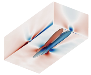
Uniform grid spacing is used in the spanwise direction, and hyperbolic sine stretching is applied in the wall-normal direction. The grid spacing is uniform in the streamwise direction except at the end of the computational domain where stretching is applied. The parameters of simulation are shown in table 1. The grid resolutions used are comparable to other reliable DNSs of compressible TBLs (Zhang, Duan & Choudhari 2017; Bernardini et al. 2021; Huang et al. 2022; Xu et al. 2022). A higher resolution is achieved in M8T05 to capture finer turbulent structures. Various first- and second-order flow statistics have been validated by matching reference data in our previous work (Zhang et al. 2022b), verifying the sufficiency of grid resolutions. The number of flow fields and the period for statistics are enough for statistical convergence. The computational domain and vortical structures are plotted in figure 1. The vortical structures near the outlet are damped by the stretched grid and the buffer zone. The regions of fully developed flows are selected for analysis as $x/\delta _i\in [24.1,48.4]$ for M2T05 and $x/\delta _i\in [27.8,44.4]$ for M8T05, respectively, as highlighted in colours in figure 1. These regions are selected according to the distribution of the Reynolds analogy factor, which will be discussed in the following section. Parameters and statistical properties of the boundary layers at the centre locations of these domains are listed in table 2. The two boundary layers are compared based on very close friction Reynolds numbers ${\textit {Re}}_\tau$. The isothermal-wall temperature $T_w$ of both TBLs are set based on the same ratio $T_w/T_r=0.5$, where the recovery temperature is defined as $T_{r}=T_{\infty }(1+r(\gamma -1) M^{2} / 2)$ based on a recovery factor of $r=0.89$ (Zhang, Duan & Choudhari 2018). Meanwhile, the non-dimensional wall heat fluxes $-B_q$ are comparable in both cases.

Table 1. The parameters of simulations: $N_x$, $N_y$ and $N_z$ are the numbers of grid points in three directions; $L_x$, $L_y$ and $L_z$ are the lengths of the physical computational domain based on the inlet boundary-layer thickness $\delta _i$; $\Delta x^+$ and $\Delta z^+$ represent streamwise and spanwise grid spacings in the wall unit, respectively; $\Delta y^+_w$ and $\Delta y^+_e$ represent the wall-normal grid spacings at the wall and the boundary edge, respectively; $N_f$ is the number of flow fields sampled for statistics and $t_su_\infty /\delta _i$ is the period for ensemble averaging.

Figure 1. Computational domain and vortical structures illustrated by isosurface of $Q$-criterion. The domains selected for analysis are colourfully flooded by the streamwise velocity.

Table 2. Parameters and statistical properties of the boundary layers at the centre location of the domain selected for analysis: $M=u_\infty /c_\infty$ and $T_\infty$ are the free stream Mach number and temperature, respectively; ${\textit {Re}}_\delta =\rho _{\infty }u_\infty \delta /\mu _\infty$ is the Reynolds number based on the boundary-layer thickness; ${\textit {Re}}_\tau =\bar {\rho }_w u_\tau \delta / \bar {\mu }_{w}$ is the friction Reynolds number. The Reynolds numbers based on the momentum thickness are ${{\textit {Re}}}_{\theta }=\rho _{\infty } u_{\infty } \theta / \mu _{\infty }$ and ${{\textit {Re}}}_{\delta _{2}}=\rho _{\infty } u_{\infty } \theta / \bar {\mu }_{w}$. Additionally, $\mathcal {H}=\delta ^{*} / \theta$ is the shape factor; $B_{q}=-(\mathrm {d} \bar {T} / \mathrm {d}y^+)_w / {\textit {Pr}} T_w$ indicates the non-dimensional wall heat flux; $T_w/T_r$ means the ratio of isothermal-wall temperature to recovery temperature and $\varTheta =(T_w-T_\infty )/(T_r-T_\infty )$ is the dimensionless temperature.

The database used has been well validated in our previous work (Zhang et al. 2022b), and we briefly review the results first. As shown in figure 2, compared with reference data, the distributions of $u_{vd}^+$ reasonably agree with the wall law and the log law, where the superscript $(\bullet )^+$ denotes a quantity in the wall unit. However, the wall-cooling effects make the distributions shrink slightly in the viscous sublayer and overshoot in the log layer, in accordance with Zhang et al. (2018). The density-scaled turbulent intensity and Reynolds shear stress collapse well with the reference data (Pirozzoli & Bernardini 2011; Zhang et al. 2018), with larger magnitudes for M8T05 in the outer layer.

Figure 2. Statistical properties: (a) van Driest transformed mean velocity $u_{vd}^+$; (b) density-scaled turbulent intensity and Reynolds shear stress. $- {\cdot } - {\cdot } -$, wall law $u^+_{vd}=y^+$; $---$, log law $u^+_{vd}=\log {(y^+)}/k+C$ with $k=0.41$, $C=5.2$.

The simulation accuracy of the thermodynamic process is also confirmed by the faithful validation of velocity-temperature statistical properties shown in figure 3. The model of Zhang et al. (2014) is able to accurately predict the relation between mean temperature and velocity, while deviation is observed in the result of the equation of Walz (1969). Since the viscous heating and the development of the boundary layer are strongly coupled, the strong Reynolds analogy (SRA) allows the correlations that the velocity-temperature correlation coefficient $R_{uT}=-1$ and the turbulent Prandtl number ${\textit {Pr}}_t=1$, as long as the total temperature fluctuations are negligible (Morkovin 1962). As depicted in figure 3(b), in the highly cooled cases, it is obtained that $R_{uT}\approx 1$ near the wall, instead of the perfect anticorrelation between velocity and temperature fluctuations indicated by SRA. In the inner layer, $R_{uT}$ is sensitive to the temperature ratio $T_w/T_r$; in the outer layer, $R_{uT}$ shows a asymptotic behaviour of $-R_{uT}\approx 0.55$ (Huang et al. 2022). The turbulent Prandtl numbers ${\textit {Pr}}_t$ are consistent with the reference data (Zhang et al. 2018) in figure 3(c). A reasonable prediction in the outer region of boundary layers can be provided by the linear relation ${\textit {Pr}}_t=1-(y/\delta )/4$ proposed by Subbareddy & Candler (2011). Moreover, the modified SRA of Huang et al. (1995) (HSRA) is plotted in figure 3(d). The distributions of the present two cases are close to unity in the outer region of boundary layers and in agreement with the reference data (Duan, Beekman & Martín 2010; Huang et al. 2022).

Figure 3. Velocity-temperature statistical properties: (a) the distribution of mean temperature $\bar {T}/T_\infty$ versus mean velocity $\bar {u}/u_\infty$; (b) the velocity-temperature correlation coefficient $-R_{uT}$; (c) the turbulent Prandtl number ${\textit {Pr}}_t$; (d) the modified SRA of Huang, Coleman & Bradshaw (1995).

3. Overall wall shear stress and heat flux

To depict a general picture of WSS and WHF in the supersonic and hypersonic TBLs, we begin by introducing the fundamental statistical and instantaneous properties in this section. Because of the strongly positive correlation of near-wall velocity and temperature fields shown in figure 3(b), the extreme events of WSS and WHF are probably related to the similar structures. For a more direct comparison, referring to Tong et al. (2022), the WSS and WHF are defined as

(3.1a,b)\begin{equation} \tau_w(x, z, t)=\left.\mu \frac{\partial u(x, y, z, t)}{\partial y}\right|_{y=0},\quad q_w(x, z, t)=\left.k \frac{\partial T(x, y, z, t)}{\partial y}\right|_{y=0}. \end{equation}

The definition of $q_w$ is analogous to that of $\tau _w$ with the same direction of the gradient, which is different to the conventional form. Figure 4 shows the distributions of the skin-friction coefficient $C_f=2 \bar {\tau }_w /(\rho _{\infty } u_{\infty }^2)$, heat-transfer coefficient $C_h=\bar {q}_w /(\rho _{\infty } u_{\infty } c_p(T_r-T_w))$ and Reynolds analogy factor $s=2C_h/C_f$ as a function of the Reynolds number $Re_\theta$. Two commonly used incompressible relations of $C_{f,i}$, namely the Kármán–Schoenherr relation (Roy & Blottner 2006) and modified Coles–Fernholz relation (Nagib et al. 2007), are transformed for comparison, written as

(3.2)$$\begin{gather} \left(C_{f, i}\right)_{K S}=\left(\log _{10}\left(2 R e_{\theta i}\right) \left[17.075 \log _{10}\left(2 Re_{\theta i}\right)+14.832\right]\right)^{-1}, \end{gather}$$

(3.3)$$\begin{gather}\left(C_{f, i}\right)_{C F}=2\left(2.604 \log R e_{\theta i}+4.127\right)^{-2}. \end{gather}$$

According to the van Driest II transformation (Van Driest 1956), the skin friction of compressible TBLs can be estimated in terms of skin friction models for incompressible TBLs through

(3.4a,b)\begin{equation} C_f=C_{f,i}/F_c,\quad Re_\theta=Re_{\theta,i}/F_\theta. \end{equation}

The transform coefficients $F_c$ and $F_\theta$ are

(3.5a,b)\begin{equation} F_c=\frac{T_r / T_{\infty}-1}{\left(\sin ^{-1} A+\sin ^{-1} B\right)^2},\quad F_\theta=\frac{\mu_\infty}{\mu_{w}}, \end{equation}

where $A$ and $B$ are correlated to the boundary layer parameters; refer to Rumsey (2010) and Huang et al. (2022). Both the transformed relations reasonably describe the distributions of $C_f$ in M2T05 and M8T05 with the cold wall. Specifically, the modified Coles–Fernholz relation performs better in M2T05 with ${\textit {Re}}_{\theta }\sim O(1\times 10^3)$, while the Kármán–Schoenherr relation has higher accuracy in M8T05 with ${\textit {Re}}_{\theta }\sim O(1\times 10^4)$. The Reynolds analogy factor is almost a constant $s\approx 1.14$ in the fully developed turbulent region for both cases. This constant is very close to the recommended value $s=1.16$ by Chi & Spalding (1966) and Hopkins & Inouye (1971). In region (i), the turbulence is initialized by the recycling/rescaling inflow boundary condition, and in region (iii), the turbulence is damped by the buffer zone near the outlet. Thus, the domain for the following analysis is selected as region (ii), which guarantees a well-developed turbulent behaviour as it has far enough distance from region (i) and region (iii).

Figure 4. Skin-friction coefficient $C_f$, heat-transfer coefficient $C_h$ and Reynolds analogy factor $s=2C_h/C_f$ versus Reynolds number $Re_\theta$ for the cases (a) M2T05, (b) M8T05. The dashed line indicates $s=1.14$, the symbols denote the incompressible relations of Kármán–Schoenherr (Roy & Blottner 2006) and Coles–Fernholz (Nagib, Chauhan & Monkewitz 2007) transformed by the van Driest II transformation. The lightly shaded regions (i) and (iii) mark the boundary layer developing region and the region influenced by buffer zone, respectively, and the shaded regions (ii) mark the domains selected for analysis.

Figure 5(a) shows the p.d.f.s of normalized WSS and WHF fluctuations $\tau _w^\prime /\tau _{w,rms}$ and $q_w^\prime /q_{w,rms}$, where $\tau _{w,rms}$ and $q_{w,rms}$ are the root mean squares of WSS and WHF fluctuations, respectively. The distributions of p.d.f.s are consistent with a TBL of $M=2.25$ and $T_w/T_r=0.75$ (Tong et al. 2022), except for the negative tails. It is seen that the negative tails in M2T05 are suppressed by wall cooling, and strong viscous heating in M8T05 promotes the extreme heat transport to the wall. Generally, in both cases, the probabilities of the positive tails are significantly higher than those of the negative tails, and the profiles are highly positively skewed. As shown in table 3, the skewnesses of $\tau _w^\prime$ and $q_w^\prime$ for both cases are positive, with the value approximating 1.0 except for $S_\tau$ of M8T05. In addition, the flatness $F_q$ of M8T05 is much larger than that of M2T05, indicating much stronger intermittency in the $q_w^\prime$ fluctuation field for M8T05; thus, more intense extreme events of $q_w^\prime$ in M8T05 are expected. If the EP and EN events are defined by the same constant threshold as in the previous work (Pan & Kwon 2018; Tong et al. 2022), it will result in the number of EP events being far more than the number of EN events. Moreover, there has been no consensus on defining the threshold for extreme events (Guerrero et al. 2020). For the purpose of relevant comparisons and ensuring that the fluctuations in extreme events are extremely positive or negative, we define the EP/EN events as the strong positive or negative fluctuations in the first $1\,\%$, respectively, which are marked by the shades in figure 5(a). In other words, the thresholds are chosen by making EP/EN events occupy a fixed percentage of total events, i.e. $\varepsilon =1\,\%$ in the present analysis. The thresholds of EP/EN events $(\phi _{tp}^\prime, \phi _{tn}^\prime )$ can be determined by setting that the integral equations of p.d.f.s are satisfied as

(3.6a,b)\begin{equation} \int_{\phi_{tp}^\prime}^{\phi^\prime_{max}}\mathcal{F}\left(\phi^\prime\right) {\rm d} \phi^\prime=\varepsilon,\quad \int_{\phi^\prime_{min}}^{\phi_{tn}^\prime}\mathcal{F}\left(\phi^\prime\right) {\rm d} \phi^\prime=\varepsilon, \end{equation}

where $\phi ^\prime$ can represent the WSS/WHF fluctuations $(\tau _w^\prime, q_w^\prime )$, and $\mathcal {F}(\phi ^\prime )$ is the p.d.f. of the fluctuations. The specific thresholds of EP and EN events obtained are shown in table 4.

Figure 5. P.d.f.s of $\tau _w^\prime /\tau _{w,rms}$ and $q_w^\prime /q_{w,rms}$: (a) the distributions of single point p.d.f.s; the distributions of joint p.d.f.s for (b) M2T05 and (c) M8T05. The diamond and circle symbols indicate the p.d.f.s of $\tau _w^\prime$ and $q_w^\prime$ in Tong et al. (2022) with $M=2.25$ and $T_w/T_r=0.75$, respectively. The shades mark the fluctuations belonging to extreme events. The values of joint p.d.f.s increase as the contour colours change from blue to red.

Table 3. Statistics of WSS and WHF fluctuations: root-mean-square value $\phi _{rms}=\sqrt {\phi ^{\prime 2}}$, skewness $S_\phi =\overline {\phi ^{\prime 3}} /(\overline {\phi ^{\prime 2}})^{3 / 2}$ and flatness $F_\phi =\overline {\phi ^{\prime 4}} /(\overline {\phi ^{\prime 2}})^2$.

Table 4. Thresholds of extreme events for WSS and WHF fluctuations.

Regarding the joint p.d.f.s depicted in figure 5(b,c), the most probable combination of ($\tau _w^\prime$, $q_w^\prime$) emerges in the third quadrant for both cases because of the cold-wall condition. Obviously, the distribution of the joint p.d.f. for M2T05 shows a very elongated shape, i.e. $\tau _w^\prime$ and $q_w^\prime$ tend to be highly positively correlated, which is consistent with the correlation coefficient in figure 3(b). For M8T05, the distribution of the joint p.d.f. shows an oyster-like shape, and the negative fluctuations of $\tau _w^\prime$ and $q_w^\prime$ are more positively correlated with each other than the positive counterpart. This is probably because heat conduction plays a key role in the combination of negative fluctuations $(\tau ^\prime _w<0,q^\prime _w<0)$. For the overall flow field of M8T05, wall streaks are the main structures. Due to wall-cooling effects, low-speed streaks are more probable to induce negative $q_w^\prime$, while in high-speed streaks, other mechanisms such as viscous dissipation and convection become more important, which suppresses the correlation between $\tau _w^\prime$ and $q_w^\prime$.

To directly visualize the overall flow organization in the fields of $\tau _w^\prime$ and $q_w^\prime$, we plot the instantaneous fluctuating fields in figure 6. The additional purple and green colour scales are used to indicate EP and EN events, respectively. The $\tau _w^\prime$ field of M2T05 shown in figure 6(a) is organized into elongated streamwise streaks of spanwise alternating positive and negative $\tau _w^\prime$, closely resembling the typical streaky patterns of velocity fields widely observed within incompressible and compressible TBLs (Jiménez et al. 2010; Pirozzoli & Bernardini 2011). The $q_w^\prime$ field shown in figure 6(b) is very similar to the $\tau _w^\prime$ field, which is predictable based on the results of the joint p.d.f., implying the dominant role of heat conduction through the cold wall for M2T05. As enlarged in the upper panels, the flow structures associated with extreme events are mainly elongated streaks. Both EP and EN events of $\tau _w^\prime$ and $q_w^\prime$ are favourable to emerge under high- and low-speed streaks, respectively. For M8T05, the fields of $\tau _w^\prime$ and $q_w^\prime$ are more complicated. Apart from the typical flow structure of streaks, the travelling-wave-like APNSs are observed in both fluctuating fields. APNSs show a spotty form with a fine spatial scale, whose streamwise scale is far smaller than that of streaks. This kind of structure has been reported in high-speed wall-bounded turbulent flows in which compressibility plays a significant role, such as in channels (Yu et al. 2019; Tang et al. 2020) and boundary layers (Duan et al. 2010; Xu et al. 2021). APNSs were found to be closely related to dilatational motions and contribute to pressure fluctuations significantly (Zhang et al. 2022b). Generally, APNSs tend to concentrate within the cold low-speed streaks (Tang et al. 2020), in which the local sound speed is low enough, and the acoustic mode is strong enough to permit the cold streaks to act as the ‘acoustic wave guides’ (Coleman, Kim & Moser 1995). According to the results of stability analysis, APNSs tend to emerge in the cases of higher Mach numbers and lower wall temperatures (Hu & Zhong 1998; Tang et al. 2020). It is noteworthy that in the enlarged upper panels, these two kinds of flow structures, i.e. APNSs and streaks, are able to induce extreme events. An overall comparison shows that streaks seem to dominate in extreme events of $\tau _w^\prime$, while APNSs seem to dominate in extreme events of $q_w^\prime$.

Figure 6. Instantaneous fluctuating fields of (a,c) $\tau _w^\prime /\tau _{w,rms}$ and (b,d) $q_w^\prime /q_{w,rms}$, for (a,b) M2T05 and (c,d) M8T05. The purple and green colour scales indicate EP and EN events, respectively. Two types of flow structures associated with extreme events, namely the streak and APNS, are enlarged in the upper panels for a clearer observation.

Given the scale difference of streaks and APNSs, to show the spectral characteristics of $\tau _w^\prime$ and $q_w^\prime$, two-dimensional pre-multiplied wavenumber spectra $k_xk_z\varPhi ^+(\lambda _x^+,\lambda _z^+)$ with integrated one-dimensional pre-multiplied wavenumber spectra $k_x\phi ^+(\lambda _x^+)$ and $k_z\phi ^+(\lambda _z^+)$ are plotted in figure 7. For M2T05, as shown in figure 7(a,b), the spectra of $\tau _w^\prime$ and $q_w^\prime$ are quite similar to each other, yielding almost the same peak wavelengths of $\lambda _x^+\approx 1200$ and $\lambda _z^+\approx 150$ indicated by the dash lines. These length scales agree with the typical near-wall streaks in the inner layer, reported in the incompressible TBLs (Hutchins & Marusic 2007) and compressible TBLs (Pirozzoli & Bernardini 2013). In addition, the wall-cooling effects increase the coherence of flow structures, and the spanwise peak wavelength becomes larger than the adiabatic case $\lambda _z^+\approx 100$ which is also consistent with the trend found by Coleman et al. (1995). The characteristics of spectra become much more different for M8T05, as depicted in figure 7(c,d). Two local peaks are observed with nearly the same spanwise wavelength $\lambda _z^+\approx 150$ as well as two distinct streamwise wavelengths $\lambda _x^+\approx 80$ and $\lambda _x^+\approx 900$. Accordingly, the peaks with finer and larger streamwise wavelengths are induced by APNSs and near-wall streaks, respectively. Due to the feature that APNSs prefer to concentrate within the low-speed streaks, the spanwise wavelengths of these two peaks are close. Consistent with the direct observation in figure 6(c,d), in the spectrum of $\tau _w^\prime$, the dominant peak originates from streaks with $\lambda _x^+\approx 900$, while in the spectrum of $q_w^\prime$, the dominant peak shifts to originate from APNSs with $\lambda _x^+\approx 80$. This double-peak feature of wall quantity spectra has also been found in high-speed cooled channel flows (Yu et al. 2022) with bulk Mach number up to 4.79, implying that this is a general effect of the strong compressibility.

Figure 7. Two-dimensional pre-multiplied wavenumber spectra $k_xk_z\varPhi ^+(\lambda _x^+,\lambda _z^+)$ with integrated one-dimensional pre-multiplied wavenumber spectra $k_x\phi ^+(\lambda _x^+)$ (top) and $k_z\phi ^+(\lambda _z^+)$ (right) of (a,c) $\tau _w^\prime$ and (b,d) $q_w^\prime$ for (a,b) M2T05 and (c,d) M8T05. The dashed lines correspond to the peak values in the one-dimensional spectra.

4. Conditional analysis on extreme events

In this section, to investigate the coherent structures associated with extreme events, we attempt to extract the coherent structures by means of volumetric conditional average at first. Then, to explore the physical mechanisms of how these coherent structures contribute to extreme $\tau _w^\prime$ and $q_w^\prime$, we propose a novel decomposition method on conditionally averaged skin-friction and heat-flux coefficients. In this manner, the contribution of the momentum and energy transport mechanisms in extreme events can be quantitatively assessed.

4.1. Conditionally averaged field based on extreme events

For identifying the coherent structures associated with specific extreme events, the volumetric conditional average is commonly used (Pan & Kwon 2018; Cardesa et al. 2019; Guerrero et al. 2020; Tong et al. 2022). The conditionally averaged quantity is denoted as $\langle \bullet \rangle (\boldsymbol {x},t)$. Referring to Pan & Kwon (2018) and Tong et al. (2022), the size of the average box is selected as $-300<\Delta x^+<300$ and $0< y^+<300$ in streamwise and wall-normal directions, respectively, as well as the whole spanwise domain for the sake of performing Helmholtz decomposition in the following. The indicative extreme $\tau _w^\prime$ and $q_w^\prime$ are set at $\Delta x^+=0$, $\Delta z^+=0$ to locate the average box. The subscripts $\langle \bullet \rangle _{EP}$ and $\langle \bullet \rangle _{EN}$ represent the conditionally averaged quantities associated with EP and EN events, respectively.

Table 5 lists the parameters and results of the conditional average. The number of extreme events $n_E$ exceeds $10^6$, guaranteeing the convergence of the conditional average. The ratios of the conditionally averaged skin-friction coefficient to the overall skin-friction coefficient $\langle C_f\rangle _{EP}/C_f$ are approximately the same for both cases, while the ratios of the conditionally averaged heat-transfer coefficient to the overall heat-transfer coefficient $\langle C_h\rangle _{EP}/C_f$ for M8T05 is much larger than that for M2T05, also implying the more intense extreme events in the $q_w^\prime$ field for M8T05. Furthermore, associated with extremely negative events, $\langle C_f\rangle _{EN}$ and $\langle C_h\rangle _{EN}$ for M8T05 become negative values, implying flow states of backflow and reverse heat transfer in the sense of conditional average. According to the conditionally averaged coefficients, it can be expected that the transports of momentum and energy in extreme events are much more intense than those in mean flow. Due to the strong positive correlation of $\tau _w^\prime$ and $q_w^\prime$ for M2T05, the fluctuations that coexist in extreme $\tau _w^\prime$ and $q_w^\prime$ events occupy the majority, resulting in the percentages of $86\,\%$ and $76\,\%$ for EP and EN events, respectively. These percentages indicate that the same flow structures, i.e. near-wall streaks, play a dominating role in both extreme $\tau _w^\prime$ and $q_w^\prime$ events. For M8T05, the overlapping percentages decrease significantly for EP events and slightly for EN events, suggesting there are different dominating flow structures associated with extreme $\tau _w^\prime$ and $q_w^\prime$ events.

Table 5. Parameters and results of conditional average: $n_E$ is the sample number of extreme events; $C_f$ and $C_h$ are the skin-friction and heat-transfer coefficients, respectively; $\langle C_f\rangle$ and $\langle C_h\rangle$ indicate the conditionally averaged skin-friction and heat-transfer coefficients, respectively; $P$ is the percentage of the events which coexist both in extreme $\tau _w^\prime$ and $q_w^\prime$ events.

Conditionally averaged $\langle \tau _w^\prime \rangle$ and $\langle q_w^\prime \rangle$ fields in the vicinity of extreme events at $\Delta x^+=0$ and $\Delta z^+=0$ are plotted in figure 8, with the white lines circling the regions belonging to extreme WSS and WHF fluctuations. For M2T05, the $\langle \tau _w^\prime \rangle$ and $\langle q_w^\prime \rangle$ fields are similar to each other. Regarding EP events, the fluctuation patterns are of elongated shapes, and the extreme regions extend to a relatively large area. Regarding EN events, the areas of extreme regions are quite small, and high-value regions are observed at two sides. However, for M8T05, only in the $\langle \tau _w^\prime \rangle _{EP}$ field is an elongated structure present. All of the extreme regions circled with white lines show spotty shapes. The streamwise structures in the $\langle \tau _w^\prime \rangle _{EN}$ field seem to be split around the extreme region, with the centre structure extending in the spanwise direction. As far as the $\langle q_w^\prime \rangle$ fields are concerned, the fine-scale alternating positive and negative patterns are shown, reminding us of the dominant role of APNSs in the extreme events of $q_w^\prime$. For the three-dimensional coherent structures associated with extreme events, they will be discussed in detail with a combination of the conditional skin-friction and heat-transfer decompositions in §§ 4.3 and 4.4.

Figure 8. Conditionally averaged $\langle \tau _w^\prime \rangle$ and $\langle q_w^\prime \rangle$ fields around extreme events at $\Delta x^+=0$ and $\Delta z^+=0$ of (a–d) M2T05 and (e–h) M8T05. The left and right panels stand for EP and EN events, respectively. The white lines circle the regions belonging to extreme WSS and WHF fluctuations.

4.2. Conditional skin-friction and heat-transfer decompositions

The skin-friction and heat-transfer decompositions based on integral identities are able to provide valuable insight into transport mechanisms contributing to WSS and WHF (Wenzel et al. 2022; Xu et al. 2022). Based on integrating the conservation laws of different quantities, such as momentum (Fukagata et al. 2002), mean kinetic energy (Renard & Deck 2016), mechanical energy (Drela 2009), total enthalpy (Wenzel et al. 2022), internal energy (Xu et al. 2022) and so on, there are many kinds of different integral identities. However, all these identities are based on overall averaged equations and are proposed to describe the mean flow and corresponding transport mechanisms; some transient behaviours, such as in extreme events of $\tau _w^\prime$ and $q_w^\prime$ discussed here, cannot be taken into account in isolation yet. For depicting extreme events and demonstrating how coherent structures associated with extreme events contribute to $\tau _w^\prime$ and $q_w^\prime$, we have developed the conditional skin-friction and heat-transfer decompositions based on the conditionally averaged governing equations.

Referring to recently developed skin-friction and heat-transfer decompositions on mean flow (Wenzel et al. 2022; Xu et al. 2022), the FIK-like identity with twofold integration is adopted here, which owns a more intuitive physical interpretation of the underlying mechanisms of transferring momentum and energy than the RD and original FIK decompositions (Wenzel et al. 2022). We start from the fully compressible Navier–Stokes equations and use the conditional average on extreme events, so that the corresponding physical mechanisms associated with extreme $\tau _w^\prime$ and $q_w^\prime$ can be particularly assessed. In combination with the continuity equation, the conditionally averaged streamwise-momentum equation can be written as

(4.1)\begin{equation} \left\langle\rho\right\rangle\frac{\partial \tilde{u}}{\partial t}+ \left\langle\rho\right\rangle\tilde{u}_j\frac{\partial \tilde{u} }{\partial x_j}+ \frac{\partial \left\langle\rho\right\rangle \widetilde{u^{\prime \prime} u_j^{\prime \prime}}}{\partial x_j}=-\frac{\partial \left\langle \,p\right\rangle}{\partial x}+\sqrt{\gamma}\frac{ M}{{\textit{Re}}} \frac{\partial \langle\tau_{1 j}\rangle}{\partial x_j}, \end{equation}

where the symbol $\widetilde {(\bullet )}$ denotes the conditional Favre average $\tilde {\phi }=\langle \rho \phi \rangle /\langle \rho \rangle$, the symbol $(\bullet )^{\prime \prime }$ denotes the fluctuation in the context of the conditional Favre average $\phi ^{\prime \prime }=\phi -\tilde {\phi }$. Based on the FIK-like identity, the conditionally averaged skin-friction coefficient can be decomposed as

(4.2)\begin{equation} \left\langle C_f\right\rangle=C_f^M+C_f^T+C_f^P+C_f^B+C_f^U, \end{equation}

specifically,

(4.3)$$\begin{gather} C_f^M=-\frac{1}{q_{\infty} y_b} \int_0^{y_b}\left(y_b-y\right) \langle\rho\rangle \tilde{u}_j \frac{\partial \tilde{u} }{\partial x_j} {{\rm d}y}, \end{gather}$$

(4.4)$$\begin{gather}C_f^T=-\frac{1}{q_{\infty} y_b} \int_0^{y_b}\left(y_b-y\right)\left(\frac{\partial\langle\rho\rangle \widetilde{ u^{\prime \prime} u^{\prime \prime}} }{\partial x}+\frac{\partial\langle\rho\rangle \widetilde{ u^{\prime \prime} w^{\prime \prime}} }{\partial z}\right)+\langle\rho\rangle \widetilde{ u^{\prime \prime} v^{\prime \prime}} {{\rm d}y}, \end{gather}$$

(4.5)$$\begin{gather}C_f^P=-\frac{1}{q_{\infty} y_b} \int_0^{y_b}\left(y_b-y\right) \frac{\partial\langle \,p\rangle}{\partial x} {{\rm d}y}, \end{gather}$$

(4.6)$$\begin{gather}C_f^B=\frac{1}{q_{\infty} y_b} \frac{\sqrt{\gamma} M}{\operatorname{{\textit{Re}}}} \int_0^{y_b}\left(y_b-y\right)\left(\frac{\partial\left\langle\tau_{x x}\right\rangle}{\partial x}+\frac{\partial\left\langle\tau_{x z}\right\rangle}{\partial z}\right)+\left\langle\tau_{x y}\right\rangle {{\rm d}y}, \end{gather}$$

(4.7)$$\begin{gather}C_f^U=-\frac{1}{q_{\infty} y_b} \int_0^{y_b}\left(y_b-y\right)\langle\rho\rangle \frac{\partial \tilde{u} }{\partial t} {{\rm d}y}, \end{gather}$$

where $q_\infty =\rho _{\infty }u_\infty ^2/2$ is the dynamic pressure and $y_b$ denotes the upper bound of integrals. According to the physical meanings of the integrands, each term can be interpreted as: $C_f^M$ is the mean-convection term; $C_f^T$ is the turbulent-convection term; $C_f^P$ is the pressure-gradient term; $C_f^B$ is the boundary-layer term and $C_f^U$ is the unsteady term.

In the same way, based on the conditionally averaged internal energy equation

(4.8)\begin{align} \left\langle\rho\right\rangle\frac{\partial \tilde{T}}{\partial t}+ \left\langle\rho\right\rangle\tilde{u}_j\frac{\partial \tilde{T} }{\partial x_j}+ \frac{\partial \left\langle\rho\right\rangle \widetilde{ T^{\prime \prime} u_j^{\prime \prime}}}{\partial x_j}=-\frac{1}{c_v}\left\langle \,p \frac{\partial u_j}{\partial x_j}\right\rangle+\frac{\sqrt{\gamma}}{c_v} \frac{ M}{ {\textit{Re}}}\left\langle \tau_{i j} \frac{\partial u_i}{\partial x_j}\right\rangle+ \frac{1}{c_v \alpha} \frac{\partial}{\partial x_j}\left\langle\mu \frac{\partial T}{\partial x_j}\right\rangle\!, \end{align}

the conditionally averaged heat-transfer coefficient can be decomposed as

(4.9)\begin{equation} \left\langle C_h\right\rangle=C_h^M+C_h^T+C_h^P+C_h^V+C_h^B+C_h^U, \end{equation}

specifically,

(4.10)$$\begin{gather} C_h^M=-\frac{c_v}{\beta y_b} \int_0^{y_b}\left(y_b-y\right) \langle\rho\rangle \tilde{u}_j \frac{\partial \tilde{T} }{\partial x_j} {{\rm d}y}, \end{gather}$$

(4.11)$$\begin{gather}C_h^T=-\frac{c_v}{\beta y_b} \int_0^{y_b}\left(y_b-y\right)\left(\frac{\partial\langle\rho\rangle \widetilde{ T^{\prime \prime} u^{\prime \prime}} }{\partial x}+\frac{\partial\langle\rho\rangle \widetilde{ T^{\prime \prime} w^{\prime \prime}} }{\partial z}\right)+\langle\rho\rangle \widetilde{ T^{\prime \prime} v^{\prime \prime}} {{\rm d}y}, \end{gather}$$

(4.12)$$\begin{gather}C_h^P=-\frac{1}{\beta y_b} \int_0^{y_b}\left(y_b-y\right) \left\langle \,p \frac{\partial u_j}{\partial x_j}\right\rangle {{\rm d}y}, \end{gather}$$

(4.13)$$\begin{gather}C_h^V=\frac{1}{\beta y_b} \frac{\sqrt{\gamma} M}{{\textit{Re}}} \int_0^{y_b}\left(y_b-y\right)\left\langle\tau_{i j} \frac{\partial u_i}{\partial x_j}\right\rangle {{\rm d}y}, \end{gather}$$

(4.14)$$\begin{gather}C_h^B=\frac{c_v}{\beta y_b} \frac{1}{c_v \alpha} \int_0^{y_b}\left(y_b-y\right)\left(\frac{\partial}{\partial x}\left\langle\mu \frac{\partial T}{\partial x} \right\rangle +\frac{\partial}{\partial z}\left\langle\mu \frac{\partial T}{\partial z} \right\rangle \right)+\left\langle\mu\frac{\partial T}{\partial y}\right\rangle {{\rm d}y}, \end{gather}$$

(4.15)$$\begin{gather}C_h^U=-\frac{c_v}{\beta y_b} \int_0^{y_b}\left(y_b-y\right)\langle\rho\rangle \frac{\partial \tilde{T} }{\partial t} {{\rm d}y}, \end{gather}$$

where the parameter $\beta$ is defined as $\beta =\rho _{\infty } u_{\infty } c_p(T_r-T_w)$. Similarly, each term can be interpreted according to the physical meanings of the integrands as: $C_h^M$ is the mean-convection term; $C_h^T$ is the turbulent-convection term; $C_h^P$ is the pressure-dilatation term; $C_h^V$ is the viscous-dissipation term; $C_h^B$ is the boundary-layer term and $C_h^U$ is the unsteady term. The detailed derivations of the conditional skin-friction and heat-transfer decompositions are given in Appendix B. Note that compared with the conventional skin-friction and heat-transfer decomposition based on spanwise homogeneous and mean flow (Wenzel et al. 2022; Xu et al. 2022), the main differences are that some spanwise-gradient terms and unsteady terms are still retained in the present decompositions. Particularly, the accuracy of the conditional skin-friction and heat-transfer decompositions has been verified in Appendix C.

4.3. Conditional analysis on extreme events of wall shear stress

In this subsection, the above-introduced volumetric conditionally averaged fluctuation fields, in combination with the proposed decomposition identities, are used to analyse the coherent structures and their corresponding momentum and energy transport mechanisms in extreme events. Figure 9 shows the conditional analysis results on extreme $\tau _w^\prime$ events for M2T05. In figure 9(a), a pair of energetic counter-rotating quasi-streamwise vortices is identified by the isosurface of $Q$-criterion coloured by the streamwise vorticity $\omega _x$. These vortices induce strong sweep motions that facilitate high-speed flow from the outer layer to the inner layer. Consequently, a high-speed streak shown by the isosurface of $u^+=2.5$ coloured by the wall-normal velocity $v$ is centred between the counter-rotating vortices near the wall. This isosurface evolves from thin to wide and to thin again along the streamwise direction, which indicates the local streamwise velocity gradient changes from positive to negative, as shown in the $x$–$y$ plane shifted from $\Delta z^+=0$. In the view of quadrant analysis (Wallace 2016), these structures associated with EP events of $\tau _w^\prime$ induce a strong Q4 event. This flow topology is consistent with those observed in the incompressible TBL (Pan & Kwon 2018), pipe flow (Guerrero et al. 2020) and compressible TBL (Tong et al. 2022). These identified coherent structures are also consistent with the conceptual model proposed by Guerrero et al. (2020). Due to the orientation of rotation, it can be deduced that the counter-rotating vortex pair is composed of the legs of two individual spanwise-arranged hairpin-like vortices, which are widely present in wall-bounded turbulent flows.

Figure 9. Conditional analysis on extreme events of $\tau _w^\prime$ for M2T05: (a,b) conditionally averaged fluctuation fields, the isosurfaces of high-/low-speed streaks are flooded by $v$, the vortices displayed by the isosurfaces of $Q$-criterion are flooded by $\omega _x$. An $x$–$y$ plane at $\Delta z^+=0$ and a $y$–$z$ plane at $\Delta x^+=0$ are shifted aside for clearer observation. Components of conditionally averaged skin-friction coefficients normalized by $C_f$: (c,e) $C_f^i$; (d,f) $C_f^i(y_b)$ as a function of the upper bound of integrals. Panels (a,c,d) and (b,e,f) are for the EP and EN events, respectively.

The components of conditionally decomposed skin-friction coefficients normalized by $C_f$ are displayed in figure 9(c,e). First, the present sample numbers of extreme events used for decompositions are sufficient to achieve statistical convergence, which has been proved in Appendix D. For a detailed comparison, the components of the mean-convection term $C_f^M$ and the turbulent-convection term $C_f^T$ in three directions are shown. The legend of lines in figure 9(d,f) can refer to figure 9(c,e) in which the colour correspondences are the same. As indicated in figure 9(d), $C_f^i(y_b)$ are independent on the integral upper bounds when $y^+_b>800$, within which the choice of $y_b$ does not affect the integral results. The dominating terms are the streamwise mean-convection term $C_f^{Mx}$, wall-normal mean-convection term $C_f^{My}$, spanwise turbulent-convection term $C_f^{Tz}$ and unsteady term $C_f^{U}$, whose magnitudes reach several times that of $C_f$. Due to the streamwise evolving of the high-speed streak, the near-wall streamwise velocity gradient has a large positive value, producing the coefficient $C_f^{Mx}$ of a large negative integral value. Moreover, it is worth noting that the profile of $C_f^{U}$ seems to be similar to that of $C_f^{Mx}$ but with an opposite sign. Provided with Taylor's frozen-flow model and assuming that the flow is streamwise dominated, it is possible to derive $\partial \tilde {u}/\partial t=-u_c\partial \tilde {u}/\partial x$ with $u_c$ being the convection velocity. If the convection velocity $u_c$ satisfies $u_c=\tilde {u}$, the profiles of $C_f^{Mx}$ and $C_f^{U}$ are expected to be opposite to each other. Actually, the convection velocity is found to be consistent with the mean velocity except for very near the wall (Zhao & He 2009; Zhang, Wan & Sun 2019). Eventually, the similar profiles of $C_f^{Mx}$ and $C_f^{U}$ could be achieved. The strong sweep motions (Q4) are the key reason to induce the EP events of $\tau _w^\prime$, which transfer amounts of momentum from the outer layer to the inner layer. The large-magnitude negative $\tilde {v}$ produces the coefficient $C_f^{My}$ of a large positive integral value. In addition, the location of EP events is between the spanwise arranged energetic vortex pairs, and the coherent vortex pair in a counter-rotating state can induce strong spanwise turbulent fluctuations. Thus, as a result of the large gradient of Reynolds stress $\widetilde {u^{\prime \prime }w^{\prime \prime }}$ in the spanwise, the coefficient $C_f^{Tz}$ also becomes an important component.

The coherent structures associated with the EN events of $\tau _w^\prime$ are shown in figure 9(b). A hairpin-like vortex following a pair of counter-rotating quasi-streamwise vortices is identified. The pair of counter-rotating vortices could also be regarded as two legs of a hairpin-like vortex. The rotating directions of the vortex pair are opposite to those in the EP events. An elongated low-speed streak is centred between the counter-rotating quasi-streamwise vortices, sustained by strong ejecting motions induced by these vortices. Therefore, the region of the streak which is shown by the isosurface of $u^+=-3$ is under a Q2 event. These identified coherent structures associated with the EN events also agree with the conceptual models proposed by Sheng et al. (2009) and Guerrero et al. (2020). The extreme events tend to be located under the two continuously streamwise-arranged hairpin-like vortices. The dominating terms are partly the same as the terms of EP events: the streamwise mean-convection term $C_f^{Mx}$, wall-normal mean-convection term $C_f^{My}$, spanwise turbulent-convection term $C_f^{Tz}$ and unsteady term $C_f^{U}$. Notably, an additional dominating term is the pressure-gradient term $C_f^P$. Due to the opposite rotating direction and the difference between high- and low-speed streaks, the contributions of $C_f^{My}$ and $C_f^{Tz}$ for EN events are quantitatively opposite to their contributions for EP events. Eventually, the mechanism which contributes most to the EN events is the pressure-gradient term $C_f^P$. The two-part structures of coherent vortices are probably related to the convecting pressure wavepackets as shown in the shifted $x$–$y$ plane. The extreme events are located behind the wave valley, resulting in a large negative value of $C_f^P$.

As for coherent structures associated with the EP events of $\tau _w^\prime$ for M8T05 shown in figure 10(a), the structures are partly similar to the counterparts of M2T05. The energetic counter-rotating quasi-streamwise vortex pair and the high-speed streak centring between the vortex pair are also identified. The biggest difference is that a spanwise-extending bridge vortex located at the EP events connects the vortex pair. This vortex is related to dilatation motions, because it is induced by the upstream expansion and downstream compression motions shown by the isosurface of $\theta ^+=\pm 0.02$. These alternating negative and positive dilatational motions remind us of the presence of APNSs in M8T05 which tend to be embedded in streaks. Despite the slight increasing contribution of other terms, the dominating terms are the same as those in M2T05: the streamwise mean-convection term $C_f^{Mx}$, wall-normal mean-convection term $C_f^{My}$, spanwise turbulent-convection term $C_f^{Tz}$ and unsteady term $C_f^{U}$. The contributions of $C_f^{My}$ and $C_f^{Tz}$ are qualitatively in agreement with those in M2T05, because of the similar counter-rotating quasi-streamwise vortex pair. Due to the strong sweep motion at EP events, the momentum is transferred from the outer layer to the inner layer, and $C_f^{My}$ contributes most to extreme $\tau _w^\prime$. Here, $C_f^{Mx}$ and $C_f^{U}$ show opposite contributions compared to those in M2T05, resulting from the deceleration region located at the buffer and log layer, but the sum of their contributions is still small.

Figure 10. Conditional analysis on extreme events of $\tau _w^\prime$ for M8T05: (a,b) conditionally averaged fluctuation fields, the isosurfaces of dilatation $\theta ^+$ are flooded by itself, the isosurfaces of high-/low-speed streaks are flooded by $v$, the vortices displayed by the isosurfaces $Q$-criterion are flooded by $\omega _x$. An $x$–$y$ plane at $\Delta z^+=0$ and a $y$–$z$ plane at $\Delta x^+=0$ are shifted aside for clearer observation. Components of conditionally averaged skin-friction coefficients normalized by $C_f$: (c,e) $C_f^i$; (d,f) $C_f^i(y_b)$ as a function of upper bound of integrals. Panels (a,c,d) and (b,e,f) are for the EP and EN events, respectively.

The coherent structures associated with the EN events shown in figure 10(b) become more complex. A horseshoe-like vortex is located behind the EN event, and the two legs are also in a counter-rotating state. A brush-shaped low-speed elongated streak is above the EN events sustained by ejection motions, indicating that EN events of $\tau _w^\prime$ for M8T05 are also related to the Q2 event. A similar spanwise-extending vortex is located at the EN events, and it is also induced by strong dilatation motions. However, in contrast to the EP event, the vortex is caught by upstream compression and downstream expansion motions shown by the isosurface of $\theta ^+=\pm 0.04$. The dominating terms are only the streamwise mean-convection term $C_f^{Mx}$, wall-normal mean-convection term $C_f^{My}$ and unsteady term $C_f^{U}$. The magnitudes of these terms are relatively large, and $C_f^{U}$ even reaches nearly $20C_f$. Comparing the coherent structures in other extreme events, we find that there is no quasi-streamwise vortex pair near the EN event; thus, the contribution of the spanwise turbulent-convection term $C_f^{Tz}$ becomes much less important. On account of the acceleration in the buffer and log layers, the streamwise mean-convection term $C_f^{Mx}$ contributes to the EN events the most. This also suggests the correlation between the outer-layer large-scale structures and the inner-layer small-scale APNS. Meanwhile, the Q2 event induces momentum transport from the inner layer to the outer layer by wall-normal mean-convection $C_f^{My}$. These coherent structures make $C_f^{U}$ a dominating term to balance the contributions of $C_f^{Mx}$ and $C_f^{My}$.

Due to the co-existence of strong shear and dilatation motions, the coherent structures associated with extreme events of $\tau _w^\prime$ for M8T05 tend to be more complex than those for M2T05. To disentangle the coupled contributions of shear and dilatational motions, we perform the Helmholtz decomposition to cast the velocity $\boldsymbol {u}$ as the sum of a solenoidal part $\boldsymbol {u}_s$ and an irrotational part $\boldsymbol {u}_d$, which satisfy $\boldsymbol {\nabla } \boldsymbol {\cdot } \boldsymbol {u}_s=0$ and $\boldsymbol {\nabla } \times \boldsymbol {u}_d=0$, respectively. Based on the velocity field $\boldsymbol {u}$, these two parts can be obtained by solving Poisson equations of the vector potential $\boldsymbol {A}$ and scalar potential $\varphi$:

(4.16a,b)\begin{equation} \nabla^2 \boldsymbol{A}=-\boldsymbol{\nabla} \times \boldsymbol{u},\quad \nabla^2 \varphi=\boldsymbol{\nabla}\boldsymbol{\cdot} \boldsymbol{u}. \end{equation}

Subsequently, the solenoidal and dilatational components can be calculated by

(4.17a,b)\begin{equation} \boldsymbol{u}_s=\boldsymbol{\nabla} \times \boldsymbol{A}, \quad \boldsymbol{u}_d=\boldsymbol{\nabla} \varphi. \end{equation}

Complemented with the boundary conditions (Hirasaki & Hellums 1970)

(4.18a–c)\begin{equation} \frac{\partial \varphi}{\partial y}=0,\quad \frac{\partial A_y}{\partial y}=0,\quad A_x=A_z=0, \end{equation}

the vector potential $\boldsymbol {A}$ is shown to be unique. Figure 11(a) shows the $\langle u\rangle _{EP}$ field at the $\Delta z^+=0$ plane, with an elongated high-speed region locating near the wall. After the Helmholtz decomposition, the structures are clearly found to be composed of the high-speed streak exhibited in figure 11(c) by the solenoidal component $\langle u_s\rangle _{EP}$ and the APNSs exhibited in figure 11(e) by the dilatational component $\langle u_d\rangle _{EP}$. The high-speed streak denoted by $\langle u_s\rangle _{EP}$ is consistent with the original coherent structures observed in incompressible pipe flow (Guerrero et al. 2020) and supersonic TBL (Tong et al. 2022) in the EP event of $\tau _w^\prime$; thus, the APNSs denoted by $\langle u_d\rangle _{EP}$ are additional structures caused by the compressible effects in high-Mach-number flow. Nonetheless, the magnitude of APNSs is an order of magnitude smaller than that of the high-speed streak. As for EN events, similarly and more apparently, the structures are also composed of the low-speed streak exhibited in figure 11(d) by $\langle u_s\rangle _{EN}$ and the APNSs exhibited in figure 11(f) by $\langle u_d\rangle _{EN}$. The difference is that the low-speed streak is thicker in the wall-normal direction, and the magnitude of the APNSs becomes larger, which is comparable to the magnitude of the streak. The phases of APNSs are reversed in EN and EP events, implying that EP or EN events are related to opposite dilatational motions.

Figure 11. Contours of the conditionally averaged fluctuation field of extreme $\tau _w^\prime$ events for M8T05 at $\Delta z^+=0$ plane: (a,b) the streamwise velocity $u$; (c,d) the solenoidal component $u_s$ and (d,f) the dilatational component $u_d$. Panels (a,c,e) and (b,d,f) are for EP and EN events, respectively.

To illustrate the ejection and sweep motions induced by these two structures, figure 12 shows contours of conditionally averaged wall-normal velocity at the $y^+=15$ plane. The strong sweep motion is observed near the location of extreme events in figure 12(a). The streak pattern in the $\langle v_s\rangle _{EP}$ field shown in figure 12(c) is more well shaped and extends longer than that in figure 12(a). Two ejecting regions simultaneously induced by the quasi-streamwise vortex pair flank the central sweeping region. The $\langle v_d\rangle _{EP}$ field in figure 12(e) shows the appearance of APNSs also with a relatively small magnitude. As for EN events, the structures in the $\langle v\rangle _{EP}$ field shown in figure 12(b) are split into several parts by weak and strong ejection motions along the $x$ direction, which consist of local ejection spots and elongated streaks. In the $\langle v_s\rangle _{EN}$ field shown in figure 12(d), the upstream ejection streak shrinks at $\Delta x^+\approx 15$ first, and then grows to be elongated. In the $\langle v_d\rangle _{EN}$ field shown in figure 12(f), the strong APNSs are identified, resulting in streamwise alternating sweeping and ejection motions. The spanwise and streamwise length scales of APNSs are consistent with the characteristic wavelength of the inner peak in figure 7(c). The APNSs also enhance ejection motions at the location of EN events. Moreover, there are phase differences in APNSs between the $u_d$ field and $v_d$ field. Similarly, Yu et al. (2019) performed Helmholtz decomposition to study compressibility effects on skin friction in turbulent channel flow. Through a modified FIK decomposition, they found a relatively small contribution of dilatational component $\boldsymbol {u}_d$ (approximately $4\,\%$) to the overall skin-friction coefficient $C_f$ in the cooled channel flow of a bulk Mach number $M_b=4.4$ with the presence of APNSs. However, the dilatational component $\boldsymbol {u}_d$ plays a much more important role in extreme $\tau _w^\prime$ events.

Figure 12. Contours of the conditionally averaged field based on extreme $\tau _w^\prime$ events for M8T05 at the $y^+=15$ plane: (a,b) the wall-normal velocity $v$; (c,d) the solenoidal component $v_s$; (e,f) the dilatational component $v_d$. Panels (a,c,e) and (b,d,f) are for EP and EN events, respectively.

4.4. Conditional analysis on extreme events of wall heat flux

Similarly, extreme $q_w^\prime$ events are analysed in the same framework. According to the joint p.d.f. in figure 5(b) where the $q_w^\prime$ is nearly linearly positively correlated with the $\tau _w^\prime$, the extreme events of $\tau _w^\prime$ and $q_w^\prime$ are mostly overlapped with each other for M2T05 referring to the overlapping percentages in table 5. Thus, the coherent structures associated with the EP events of $q_w^\prime$ shown in figure 13(a) are quite similar to those of $\tau _w^\prime$ shown in figure 9(a). A high-temperature elongated streak shown by the isosurface of $T^+=4$ centring between the counter-rotating quasi-streamwise vortex pair is subjected to sweep motions. The isosurface of this high-temperature streak evolves from thin to wide and to thin again along the streamwise direction, which indicates that the local streamwise temperature gradient changes from positive to negative as shown in the $x$–$y$ plane shifted from $\Delta z^+=0$. The dominating contributing terms are the streamwise mean-convection term $C_f^{Mx}$, the viscous-dissipation term $C_h^V$ and the unsteady term $C_f^{U}$. The counter-rotating vortex pair inducing sweep motions enhances the near-wall shear ${\partial u}/{\partial y}$, thus the EP event of $q_w^\prime$ for M2T05 is mainly the result of strong molecular viscous heating within the viscous sublayer $(y^+<5)$.

Figure 13. Conditional analysis on extreme events of $q_w^\prime$ for M2T05: (a,b) conditionally averaged fluctuation fields, the isosurfaces of high-/low-temperature streaks are flooded by $v$, the vortices displayed by the isosurfaces of $Q$-criterion are flooded by $\omega _x$. An $x$–$y$ plane at $\Delta z^+=0$ and a $y$–$z$ plane at $\Delta x^+=0$ are shifted aside for clearer observation. Components of conditionally averaged heat-transfer coefficients normalized by $C_h$: (c,e) $C_h^i$; (d,f) $C_h^i(y_b)$ as a function of the upper bound of integrals. Panels (a,c,d) and (b,e,f) are for the EP and EN events, respectively.

For the EN event of $q_w^\prime$, the coherent structures shown in figure 13(b) are also similar to those of $\tau _w^\prime$ shown in figure 9(b). A hairpin-like vortex following a pair of counter-rotating quasi-streamwise vortices is identified, and an elongated low-temperature streak shown by the isosurface of $T^+=-4$ centres between these vortices. Under these coherent structures, there is no very dominant term as the streamwise mean-convection term $C_f^{Mx}$, the wall-normal mean-convection term $C_f^{My}$, the spanwise turbulent-convection term $C_f^{Tz}$, the viscous-dissipation term $C_h^V$, the pressure-dilatation term $C_h^P$ and the unsteady term $C_f^{U}$ all have relatively considerable contributions. Compared with the dominating terms of EP events, the magnitudes of these terms of EN events are relatively small. The near-wall molecular viscous heating is highly mitigated. As is shown in the $x$–$y$ plane shifted from $\Delta z^+=0$, streamwise extended compression and expansion motions are located near the EN event, which could be related to the convecting wavepackets within the boundary layer; thus the most important transport mechanism of energy contributing to EN events becomes the pressure-dilatation work $C_h^P$.

The scenario in extreme events of $q_w^\prime$ for M8T05 is quite different. The coherent structures associated with extreme events shown in figure 14(a,b) are formed by local fine-scale spanwise-extending spotty structures near the wall, without the presence of the elongated velocity/temperature streaks and counter-rotating quasi-streamwise vortex pair observed in other extreme events. Intuitively, these dilational spanwise-extending spotty structures correspond to the APNSs directly observed in figure 6(d). The length scale of these structures is also consistent with the corresponding wavelength of the dominant spectral peak in figure 7(d). For the EP event, a fine-scale spanwise extending vortex with negative spanwise vorticity $(\omega _z<0)$ is induced by the upstream expansion and downstream compression shown by isosurfaces of $\theta ^+=\pm 0.07$, respectively. The EP events are favourable to occur behind the inflection points of APNSs where expansion transitions to compression. A vortex sheet with $(\omega _z>0)$ off the wall in the buffer layer is located downstream of the EP event. The high-temperature region of $T^+=2$ becomes a tiny isolated wall-mounted spot at the location of EP events. The dominant energy transport mechanisms seem to be much simpler than those in M2T05, the streamwise convection of the strong APNSs dominates due to their feature of convecting wavepackets. Meanwhile, the contribution of pressure-dilatation work $C_h^P$ is comparable to that of molecular viscous heating $C_h^V$. The mean-convection term $C_h^{Mx}$ and the unsteady term $C_h^{U}$ are overwhelming on other terms and comparable to each other. Their magnitudes are very large, and can even exceed $60C_h$.

Figure 14. Conditional analysis on extreme events of $q_w^\prime$ for M8T05: (a,b) conditionally averaged fluctuation fields, the isosurfaces of dilatation $\theta ^+$ and temperature $T^+$ are flooded by themselves, the vortices displayed by the $Q$-criterion are flooded by $\omega _z$. An $x$–$y$ plane at $\Delta z^+=0$ and a $y$–$z$ plane at $\Delta x^+=0$ are shifted aside for clearer observation. Components of conditionally averaged heat-transfer coefficients normalized by $C_h$: (c,e) $C_h^i$; (d,f) $C_h^i(y_b)$ as a function of the upper bound of integrals. Panels (a,c,d) and (b,e,f) are for the EP and EN events, respectively.

For the EN event, the coherent structures are also mainly associated with the APNSs. Compared with the EP event, the signs of the spanwise vorticity of the identified vortex and the dilatation are inverse, namely a fine-scale spanwise-extending near-wall vortex with positive spanwise vorticity $(\omega _z>0)$ is induced by the upstream compression and downstream expansion shown by isosurfaces of $\theta ^+\pm 0.07$. The EN events are favourable to occur behind the inflection points of APNSs where compression transitions to expansion. The low-temperature regions of $T^+=-3$ are shown to be two parts: one is also a tiny isolated wall-mounted spot at the location of EN events; another is a large-scale off-wall bubble. Similarly, the mean-convection term $C_h^{Mx}$ and the unsteady term $C_h^{U}$ are also overwhelming on other terms and comparable to each other. Compared with EP events, the growth of these two terms is slower persisting up to the wake, due to the low-temperature off-wall bubble. Meanwhile, the pressure-dilatation term $C_h^P$ is also contributive to EN events.

Since the two terms $C_h^{Mx}$ and $C_h^{U}$ are overwhelming and almost cancel each other in both EP and EN events, to more clearly compare with other mechanisms, $C_h^U$ and $C_h^{Mx}$ are combined and denoted by $C_h^{MU}=C_h^{Mx}+C_h^U$, which is a measure of comprehensive contributions by convecting structures. As shown in figure 15, the magnitudes of the combined components $C_h^{MU}$ become much smaller and comparable to other components. For EP events, the pressure-dilatation term $C_h^P$ and viscous-dissipation term $C_h^V$ play dominating roles, while $C_h^V$ is expected to be always positive; and for EN events, the dominating contribution of $C_h^P$ is highlighted. In this sense, the pressure-dilatation terms $C_h^P$, whose magnitudes grow rapidly near the wall $(y^+<10)$, have the greatest contribution to both EP and EN events. These findings are consistent with the observations of the near-wall strong-dilatation structures APNSs in the conditionally averaged field.

Figure 15. Recombined components of conditionally averaged heat-transfer coefficients for M8T05 normalized by $C_h$: (a,c) $C_h^i$; (b,d) $C_h^i(y_b)$ as a function of the upper bound of integrals. Panels (a,b) and (c,d) are for the EP and EN events, respectively.

5. Summary and conclusions

The extreme events of wall shear stress and heat flux in compressible TBLs are investigated by analysing DNS data. A supersonic case M2T05 and a hypersonic case M8T05 are considered to examine the effects of compressibility. The essential features of overall $\tau _w^\prime$ and $q_w^\prime$ have been presented at first. In both TBLs, the distribution of skin-friction coefficient $C_f$ versus Reynolds number ${\textit {Re}}_\theta$ can be properly predicted by transformed Kármán–Schoenherr and Coles–Fernholz relations. The Reynolds analogy factors are seldom influenced by the Mach number, and the values of both cases are almost the same $s\approx 1.14$. Visually indicated by the fields of $\tau _w^\prime$ and $q_w^\prime$, the primary structures associated with extreme events are high-/low-speed streaks in M2T05; in contrast, those in M8T05 become two types of distinct structures, i.e. the similar streaks and the unique fine-scale APNSs. Correspondingly, only an individual peak emerges in the wavenumber spectra with relatively longer characteristic wavelength $\lambda _x^+$ for M2T05, while two distinct peaks corresponding to APNSs and streaks are observed in the spectra with separated characteristic wavelengths $\lambda _x^+$ for M8T05. Additionally, from $\tau _w^\prime$ spectra to $q_w^\prime$ spectra, the dominating peak shifts from the peak of streaks to the peak of APNSs.

Second, the coherent structures associated with extreme events are identified by performing volumetric conditional average. In M2T05, the coherent structures involve organized hairpin-like vortices which can induce sweep/ejection events, but the conditional field becomes more complex in M8T05, and two types of coherent structures have been simultaneously identified, i.e. hairpin-like vortices and APNSs. Additionally, APNSs dominate the conditional field of extreme $q_w^\prime$ events for M8T05. Through Helmholtz decomposition, the natures of streaks and APNSs are shown to be related to solenoidal and dilatational motions, respectively. Furthermore, APNSs are found to be a type of structure capable of efficiently inducing extreme events of both $\tau _w^\prime$ and $q_w^\prime$.

Further, we propose the novel conditional skin-friction and heat-transfer decompositions based on a FIK-like identity that allows us to investigate the transport mechanisms of momentum and energy in extreme events quantitatively. The key features with respect to the transport mechanisms of these two types of coherent structures are clarified. For the hairpin-like vortices, the main transport mechanisms of momentum or energy are by the streamwise convection by speed/temperature streaks $C_f^{Mx}$ or $C_h^{Mx}$, spanwise turbulent fluctuations $C_f^{Tz}$ or $C_h^{Tz}$, and exchange of momentum or energy between the inner and outer layer by the sweep/ejection motions $C_f^{My}$ or $C_h^{My}$. It is noteworthy that in the EN events, pressure-related terms, such as the pressure-gradient term $C_f^{P}$ and the pressure-dilatation term $C_h^{P}$, are the primarily contributive terms. In contrast, for APNSs, the strong near-wall dilatational motions organized as convecting wavepackets dominate the transport of both momentum and energy by convection. Meanwhile, for energy transport, the pressure-dilatation work $C_h^P$ becomes the most contributive mechanism, in contrast to the dominant role of viscous dissipation $C_h^V$ in the viscous sublayer by the hairpin-like vortices. That is, in extreme events, the compressibility effects completely change the dominant transport mechanisms of energy by shifting the dominant flow process from transverse to longitudinal.

In short, it should be emphasized that the transport mechanisms of momentum and energy revealed above should be general since these identified streaks and APNSs are representative structures in compressible TBLs, even though the coherent structures associated with extreme events may depend on the parameters such as Mach number, temperature, etc. Of particular importance, this study offers a possible framework for analysing extreme events and corresponding transport mechanisms quantitatively by combining volumetric conditional average with the proposed conditional skin-friction and heat-transfer decompositions.