Early stage of bubble spreading in a viscous ambient liquid

Abstract

We investigate numerically the spreading dynamics of a bubble coming into contact with a smooth solid substrate in a viscous liquid. The substrate is partially wettable, and the singularity of the moving contact line is relieved by adopting the Navier-slip model. The Stokes equations are solved by employing a boundary element method coupled with adaptive mesh refinement. This allows us to realize sufficiently small slip lengths down to $O(10^{-5})$ in dimensionless form, which is crucial to resolve the local interface structures at the early stage of spreading. The results show that the early-stage spreading of the bubble is always characterized by the growth and propulsion of a dewetting liquid rim close to the contact line, while the macroscopic interface remains unchanged. The evolution of the contact line and the morphology of the rim depends on the wettability and the slip length, and a parametric investigation is performed. Based on mass conservation, a relation between the rim size and the spreading radius is established. We also propose an analytical prediction of the temporal variation in the contact line radius at the early stage of spreading, which is found to follow a logarithmically corrected linear relation rather than a pure power law. Moreover, the early stages of bubble spreading are qualitatively similar for two-dimensional and axisymmetric configurations.

1. Introduction

Interfacial flows with moving contact lines are widespread in nature and industrial applications, such as mineral flotation (Newcombe & Ralston 1994), oil recovery (Sahimi 1993), inkjet printing (Wijshoff 2018) and coating (Weinstein & Ruschak 2004), and have attracted extensive attention in recent decades (de Gennes 1985; Snoeijer & Andreotti 2013). However, the moving contact line problem contains two major difficulties that can bring great challenges to experiments and numerical simulations. One is the divergency of viscous stress in the framework of hydrodynamics coupled with no-slip conditions (Huh & Scriven 1971; Dussan & Davis 1974). A range of contact line models have been proposed to relieve contact line singularities (Bonn et al. 2009). The other difficulty is that the problem of moving contact lines is characterized by an inherently multiscale feature, involving approximately six decades of length scales from the macroscopic capillary length scale (${\sim }10^{-3}$ m) to the molecular scale (${\sim }10^{-9}$ m) (Snoeijer & Andreotti 2013).

One of the most common problems of moving contact lines is the spreading of bubbles on solid surfaces. Most investigations of bubble spreading have adopted aqueous liquids (e.g. water) as ambient fluids such that inertia effects play a dominant role. Early works have measured the contact radius or the apparent contact angle as a function of time, focusing on the effect of line tension (Stechemesser & Nguyen 1998) or the validation of various contact line models (Newcombe & Ralston 1992, 1994; Phan, Nguyen & Evans 2003). Wang et al. (2009) explored the impact of bubbles on submerged lotus leaves and reported a rapid spreading of air. The impact and subsequent spreading of a gas bubble on an aerophilic substrate was studied by de Maleprade, Clanet & Quéré (2016), who found that the spreading dynamics depended on the bubble morphologies at the first contact. When the bubble is flattened by gravity, a three-stage behaviour can be observed, with each stage characterized by a distinct scaling law. In contrast, for a spherical bubble, the contact radius grows according to the law $r(t)\sim t^{1/2}$ for both the early and late stages, although the coefficients are different. Here, r and t represent the contact radius and time, respectively. de Maleprade et al. (2016) pointed out the analogy between the early stage of bubble spreading and bubble–bubble coalescence; the short-time behaviour of bubble coalescence follows the $t^{1/2}$ law for both inviscid and viscous regimes (Paulsen et al. 2014; Munro et al. 2015; Anthony et al. 2017). In addition to the above inertia-dominated situations, the cases of viscous spreading have been experimentally investigated by employing a two-liquid system, e.g. a water drop in a highly viscous oil (Jose & Cubaud 2017; Bazazi, Sanati-Nezhad & Hejazi 2018; Jose et al. 2018). In particular, if the early stage of the spreading process is fitted according to the power law $r(t)\sim t^\beta$, then different values of $\beta$ varying from $2/3$ to 1 have been reported. Apart from the contact radius, little is known about the interfacial structures close to the contact line at the early stage of bubble spreading, which is difficult to access in prior experiments.

A problem closely related to bubble spreading is the spreading of liquid drops in air, which is analogous geometrically but with the two fluid phases exchanged. The early stage of drop spreading also follows different scaling laws depending on whether inertia or viscosity resists spreading. In the situation of low-viscosity droplets, where inertia dominates over viscous effects, Biance, Clanet & Quéré (2004) derived the power law $r(t)\sim t^{1/2}$ on completely wetting substrates. While Bird (2008) reported a wettability-dependent spreading exponent, the $t^{1/2}$ law was found to be independent of wettability and can be detected as long as sufficiently small length and time scales are resolved (Winkels et al. 2012). For spreading of drops of high viscosity, Eddi, Winkels & Snoeijer (2013) showed that the short-time spreading radius does not exhibit pure power-law growth. In both inertial and viscous regimes, the experiments of drop spreading (Biance et al. 2004; Eddi et al. 2013) suggested a similarity with the coalescence of two free drops (Eggers, Lister & Stone 1999; Wu, Cubaud & Ho 2004; Aarts et al. 2005). It remains unclear if this analogy holds for the early stage spreading of bubbles in a viscous liquid.

The present study is concerned with bubble spreading in a highly viscous liquid, adopting high-resolution numerical simulations and focusing on the spreading behaviours at the early stage. So far, a full-scale quantitative simulation of the spreading of bubbles or drops remains challenging due to the presence of a moving contact line. To alleviate the contact line singularity (Snoeijer & Andreotti 2013), various moving contact line models have been proposed, the most representative of which are the slip model (Dussan 1979), the precursor model (de Gennes 1985) and the diffuse-interface model (Seppecher 1996). Other competing contact line models have also been proposed (e.g. Shikhmurzaev 1993; Qian, Wang & Sheng 2006; Sprittles 2017; Lācis et al. 2020). All the models are characterized by a small microscopic length, which is well separated from the macroscopic length of the problem. In this study, we use the Navier-slip model (Navier 1823). For a millimetre-sized drop/bubble, the ratio of the slip length to the macroscopic characteristic length, denoted by $\lambda$, is usually $O(10^{-5})$ or less. Whilst remarkable theoretical progress has been achieved (e.g. Hocking 1983; Cox 1986; Eggers 2004, 2005; Snoeijer 2006; Chan et al. 2020), full-scale numerical simulations are still too expansive to be performed. To resolve the local flow field and the interface deformation near the contact line, the minimum mesh size should be much smaller than the slip length, leading to a prohibitively large computational cost (Sui, Ding & Spelt 2014). As a compromise, most numerical simulations of moving contact lines have been performed using unrealistically large values of slip lengths, typically $O(10^{-2})$. While qualitative wetting behaviours can be captured by these simulations, the employment of sufficiently small values of the slip length is important for making quantitative comparisons. To the best of our knowledge, available numerical simulations of moving contact lines with realistic slip lengths of $O(10^{-5})$ are typically performed using finite element methods and are only limited to two-dimensional steady situations, e.g. wetting flows in dip coating (Sprittles & Shikhmurzaev 2012; Vandre, Marcio & Satish 2012; Sprittles 2015). For unsteady flows, simulations of drop spreading for $\lambda =10^{-4}$ have been realized by Sui & Spelt (2013), who employed the level-set method coupled with parallel computing and adaptive mesh refinement. Two-dimensional finite-element calculations have been performed recently by Keeler et al. (2022), who investigated the stability of moving contact lines with slip lengths down to $10^{-4}$. In addition to the contact line singularity (Snoeijer & Andreotti 2013), there is a geometric singularity at the first contact of the bubble, corresponding to a meniscus with divergent curvature and a local dewetting film of vanishing thickness. The coupling of the two singularities brings extra challenges to numerics, and it is also crucial to employ a high-resolution approach to capture the local film structure at the early stage of spreading.

The objectives of the present work are twofold. The first is to develop a high-resolution methodology, which enables the full-scale and quantitative simulation of dynamic wetting or dewetting. The second objective is to investigate systematically the early stage behaviours of bubble spreading in a viscous liquid, with particular attention devoted to the local film structure and the existence of a scaling law. To this end, we first propose a boundary element method to simulate the spreading problem in a viscous flow. The boundary element method has also been employed by Chan et al. (2017) to study the dewetting of a viscous droplet, wherein the smallest slip length is only $O(10^{-2})$ due to the large element used. In the present method, we extend the method to two-phase systems and introduce adaptive mesh refinement to realize a large number of decades of space resolution, allowing us to handle simultaneously the small slip lengths down to $O(10^{-5})$ and the thin film at the early stage of spreading. Then this method is used to simulate the spreading of bubbles in a viscous liquid. Both two-dimensional and axisymmetric configurations will be considered. We will show that the early stage of spreading is localized in the region near the contact line and is always characterized by a dewetting rim. The employment of sufficiently small values of slip lengths enables a quantitative prediction of the small interface structure and spreading behaviours. In particular, the numerical results agree with our theoretical rationalization, which demonstrates that the spreading radius increases with time according to a logarithmically corrected linear relation.

2. Governing equations and numerical method

2.1. Governing equations

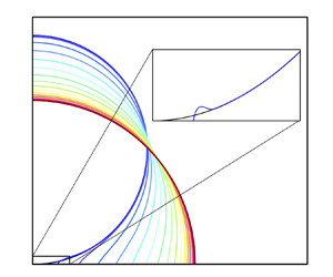
Consider a circular bubble of diameter $D_0$, which is initially brought into contact with a smooth solid substrate, as shown schematically in figure 1. The substrate is partially wettable and characterized by a finite equilibrium contact angle $\theta _e$, which is defined in the liquid phase. To minimize the surface energy, the bubble is expected to spread until it reaches the equilibrium state determined by $\theta _e$. The dynamic viscosities of the ambient liquid and the gas are denoted by $\mu$ and $M\mu$, respectively, where $M$ is the viscosity ratio. We assume that the liquid is sufficiently viscous and the bubble radius is less than the capillary length $l_c=\sqrt {\gamma /(\rho g)}$, where $\rho$, $g$ and $\gamma$ represent the liquid density, gravitational acceleration and interface tension, respectively. Accordingly, the spreading is dominated by the balance between viscous and capillary forces, and inertia and gravity can be neglected.

Figure 1. Schematic diagram of a bubble spreading on a solid. Only half of the domain is shown due to symmetry. The inset shows the geometry close to the contact line.

The problem is non-dimensionalized by rescaling all lengths by the initial diameter of the bubble $D_0$, velocities by $\gamma /\mu$, pressures and stresses by $\gamma /D_0$, and time by the visco-capillary time scale $\mu D_0/\gamma$. The flow is governed by Stokes equations, which can be written as

(2.1) \begin{equation} \left.\begin{array}{c@{}} \nabla^2 \boldsymbol{u}-\boldsymbol{\nabla} p= \boldsymbol{\nabla}\boldsymbol{\cdot}\boldsymbol{\sigma}=\boldsymbol{0},\\ \boldsymbol{\nabla}\boldsymbol{\cdot}\boldsymbol{u}= 0, \end{array}\right\} \end{equation}

in the liquid phase, and

(2.2)\begin{equation} \left.\begin{array}{c@{}} M\,\nabla^2 \boldsymbol{u}-\boldsymbol{\nabla} p=\boldsymbol{\nabla} \boldsymbol{\cdot}\boldsymbol{\sigma}=\boldsymbol{0},\\ \boldsymbol{\nabla}\boldsymbol{\cdot}\boldsymbol{u}= 0, \end{array}\right\} \end{equation}

in the gas phase, where $\boldsymbol {u}=(u_x,u_y)$ and $p$ are the velocity and pressure, respectively, and $\boldsymbol {\sigma }$ is the stress tensor.

To relieve the well-known singularity of the moving contact line, the Navier-slip condition is applied on the solid boundary. Introducing the stress force $\boldsymbol {f}\equiv \boldsymbol {\sigma }\boldsymbol {\cdot }\boldsymbol {n}$, where $\boldsymbol {n}$ is the unit normal defined in figure 1, the boundary conditions on the gas/solid boundary can be written as

(2.3a,b)\begin{equation} \boldsymbol{u}\boldsymbol{\cdot}\boldsymbol{t}=\dfrac{\lambda_1}{M}\,\boldsymbol{f}\boldsymbol{\cdot} \boldsymbol{t},\quad \boldsymbol{u}\boldsymbol{\cdot}\boldsymbol{n}=0,\end{equation}

and the boundary conditions on the liquid/solid boundary are

(2.4a,b)\begin{equation} \boldsymbol{u}\boldsymbol{\cdot}\boldsymbol{t}=\lambda_2\,\boldsymbol{f}\boldsymbol{\cdot}\boldsymbol{t},\quad \boldsymbol{u}\boldsymbol{\cdot}\boldsymbol{n}=0.\end{equation}

Here, $\boldsymbol {t}$ is the unit tangent vector of the boundary, and $\lambda _1$ and $\lambda _2$ denote the slip lengths in the gas and liquid phases, respectively. While the slip lengths can be generally different, we choose $\lambda _1=\lambda _2=\lambda$ for simplicity. The flow is assumed to vanish at the far field, i.e.

(2.5)\begin{equation} \boldsymbol{u}\rightarrow0,\quad \boldsymbol{f}\rightarrow0 \quad \mbox{as}\ \boldsymbol{x}\rightarrow\infty. \end{equation}

Across the gas/liquid interface, the velocity and the tangential stress are continuous, and the normal stress suffers a jump due to the interface tension. The total jump of the stress across the gas/liquid interface follows the Young–Laplace law

(2.6)\begin{equation} {\rm \Delta} \boldsymbol{f}\equiv\boldsymbol{f}_{g}-\boldsymbol{f}_{l}=\kappa\boldsymbol{n}, \end{equation}

where $\kappa =\boldsymbol {\nabla }\boldsymbol {\cdot }\boldsymbol {n}$ is the curvature of the gas/liquid interface, and the subscripts $g$ and $l$ denote the gas and liquid phases, respectively. The interface evolves according to the kinematic condition

(2.7)\begin{equation} \frac{\mathrm{d}\kern0.7pt\boldsymbol{x}_s}{\mathrm{d}t}=(\boldsymbol{u}\boldsymbol{\cdot}\boldsymbol{n})\boldsymbol{n}, \end{equation}

where $\boldsymbol {x}_s$ represents the location for the interface. The advantage of using normal velocity $\boldsymbol {u}\boldsymbol {\cdot }\boldsymbol {n}$ to advance the interface instead of the velocity $\boldsymbol {u}$ is that it does not need to re-mesh the interface frequently (Alinovi & Bottaro 2018).

The initial circular interface profile is described by $x^2+(y-R_0)^2=R_0^2$, where $R_0=1/2$ is the radius. This gives rise to a contact point with the substrate, representing a geometric singularity that cannot be handled numerically. To circumvent this singularity, we assume that the contact line is initially located at a small distance $r_i$ away from the symmetric axis and connects to the circle above through a small arc, which is tangent to the circle and intersects the substrate by the contact angle $\theta _e$, as shown in the inset of figure 1. The spreading is thus triggered by the large curvature of this arc. We note that this artificial initial interface profile exhibits a discontinuity of the curvature at the tangent point, which will be smoothed out in a short relaxation process. The subsequent spreading dynamics is independent of the initial position of the contact line $r_i$ provided that it is sufficiently small, as demonstrated in Appendix A. The results presented in the following are obtained by fixing $r_i=2\times 10^{-3}$, which is small enough and does not affect the interface structures of present interest. An alternative indication of the smallness of the initial contact radius is that the film thickness at $x=r_i$ confined between the unmodified circular bubble and the wall is $r_i^2=4\times 10^{-6}$, less than the smallest slip length $10^{-5}$ attained in our simulations.

The problem is thus governed by three dimensionless numbers: the equilibrium contact angle $\theta _e$, the dimensionless slip length $\lambda$, and the viscosity ratio $M$. In the present work, we focus on bubble spreading such that $M\ll 1$. In our simulations, we have fixed $M=10^{-3}$. The variation in $M$ plays a negligible role as long as it is sufficiently small (see Appendix A).

2.2. Boundary element method

We give a brief introduction to the boundary element method, which has been employed extensively to study interfacial flows (Pozrikidis 1992). The basic idea of the boundary element method is to write the governing differential equations as a set of boundary integral equations, discretize them, and finally solve the system of linear equations. The main advantage of the boundary element method is that one needs to consider the boundary distributions of only the velocities and the stresses, and flow information inside the domain is unnecessary during the calculation. This dimensionality reduction can significantly improve the calculation efficiency. Moreover, this method allows us to simulate the early stages of bubble spreading by resolving extremely small scales.

For simplicity, we begin with the spreading of two-dimensional bubbles. The boundary element method of axisymmetric cases will be discussed later. In this approach, the velocity $\boldsymbol {u}(\boldsymbol {x}_0)$ at any collocation point $\boldsymbol {x}_0$ can be written in terms of integrals involving the stress $\boldsymbol {f}$ and the velocity $\boldsymbol {u}$ on the boundary. For symmetric bubble spreading, it is necessary to employ only half of the domain, as shown in figure 1. The integral representations of the Stokes equation read

(2.8)\begin{align} & {-\frac{1}{4 {\rm \pi}}} \int_{S_1+S_2} {G_{ji}(\boldsymbol{x}_0,\boldsymbol{x})\,f_i(\boldsymbol{x})\,\mathrm{d}s (\boldsymbol{x})}+\frac{M}{4 {\rm \pi}} \int_{S_1+S_2} {u_i(\boldsymbol{x})\,T_{ijk} (\boldsymbol{x},\boldsymbol{x}_0)\,n_k(\boldsymbol{x})\,\mathrm{d}s(\boldsymbol{x})} \nonumber\\ &\quad =\left\{\begin{array}{@{}ll} M u_j(\boldsymbol{x}_0) & \text{when $\boldsymbol{x}_0$ is inside $\varOmega_g$},\\ \tfrac{1}{2}M\,u_j(\boldsymbol{x}_0) & \text{when $\boldsymbol{x}_0$ is on $S_1$ and $S_2$},\\ 0 & \text{when $\boldsymbol{x}_0$ is outside $\varOmega_g$}, \end{array}\right. \end{align}

and

(2.9)\begin{align} & {-\frac{1}{4 {\rm \pi}}} \int_{S_2+S_3} {G_{ji}(\boldsymbol{x}_0,\boldsymbol{x})\,f_i(\boldsymbol{x})\,\mathrm{d}s(\boldsymbol{x})} +\frac{1}{4 {\rm \pi}} \int_{S_2+S_3} {u_i(\boldsymbol{x})\,T_{ijk}(\boldsymbol{x},\boldsymbol{x}_0)\, n_k(\boldsymbol{x})\,\mathrm{d}s(\boldsymbol{x})} \nonumber\\ &\quad =\left\{\begin{array}{@{}ll} u_j(\boldsymbol{x}_0) & \text{when $\boldsymbol{x}_0$ is inside $\varOmega_l$},\\ \tfrac{1}{2}u_j(\boldsymbol{x}_0) & \text{when $\boldsymbol{x}_0$ is on $S_2$ and $S_3$},\\ 0 & \text{when $\boldsymbol{x}_0$ is outside $\varOmega_l$}, \end{array}\right. \end{align}

for both the gas and liquid phases, respectively. A detailed derivation of the boundary integral equations can be found in Pozrikidis (2002). As shown in figure 1, $\varOmega _g$ and $\varOmega _l$ represent the domains occupied by the bubble and the liquid, respectively. The subscripts $i,j,k$ represent either the $x$ or the $y$ component in Cartesian coordinates, and the repeated indices imply the Einstein summation convention. Here, we have implemented the vanishing flow condition (2.5), and only integrals along the gas/solid ($S_1$), gas/liquid ($S_2$) and liquid/solid ($S_3$) boundaries need to be considered. We have used the arc coordinate $s$, which increases along the direction of positive $x$ on $S_1$ and $S_3$, and away from the contact line on $S_2$. For either phase, the integrals are performed in a counterclockwise manner. Accordingly, $\mathrm {d}s<0$ along $S_2$ in (2.9). The two-dimensional velocity and stress Green's functions for symmetric Stokes flow, $G_{ij}$ and $T_{ijk}$, are given by

(2.10) \begin{equation} \left.\begin{gathered} G_{ij}(\boldsymbol{x},\boldsymbol{x}_0)=\tilde{G}_{ij}(\boldsymbol{x},\boldsymbol{x}_0)+ \tilde{G}_{im}(\boldsymbol{x},\boldsymbol{x}^*_0)\,\varLambda_{mj},\\ T_{ijk}(\boldsymbol{x},\boldsymbol{x}_0)=\tilde{T}_{ijk}(\boldsymbol{x},\boldsymbol{x}_0)+ \tilde{T}_{imk}(\boldsymbol{x},\boldsymbol{x}^*_0)\,\varLambda_{mj}, \end{gathered}\right\} \end{equation}

where we have introduced the tensor $\boldsymbol {\varLambda }= \left (\begin {smallmatrix} -1 & 0 \\ 0 & 1 \end {smallmatrix}\right )$, and $\boldsymbol {x}^*_0$ is the image of the point $\boldsymbol {x}_0$ with respect to the symmetry axis and can be expressed as $\boldsymbol {x}^*_0=\boldsymbol {\varLambda }\boldsymbol {\cdot }\boldsymbol {x}_0$. The free-space Green's functions have the form

(2.11) \begin{equation} \left.\begin{gathered} \tilde{G}_{ij}(\boldsymbol{x},\boldsymbol{x}_0)={-}\delta_{ij}\ln l+\frac{\bar{x}_i\bar{x}_j}{l^2},\\ \tilde{T}_{ijk}(\boldsymbol{x},\boldsymbol{x}_0)={-}4\,\frac{\bar{x}_i\bar{x}_j\bar{x}_k}{l^4}, \end{gathered}\right\} \end{equation}

where $\bar {\boldsymbol {x}} \equiv \boldsymbol {x}-\boldsymbol {x}_0$ and $l=|\boldsymbol {x}-\boldsymbol {x}_0|$ are the vectorial and scalar distances of the integration point $\boldsymbol {x}$ from the collocation point $\boldsymbol {x}_0$, respectively.

To embed the interfacial condition (2.6), the integral equations (2.8) and (2.9) can be summed to yield an integral representation that holds over the entire domain, similar to that used in Schleizer & Bonnecaze (1999). Specifically, the integral formulation at a point $\boldsymbol {x}_0$ located on the boundaries is written as

(2.12)\begin{align} \varPsi u_j(\boldsymbol{x}_0) &={-}\frac{1}{4{\rm \pi}}\int_{S_1}G_{ji}(\boldsymbol{x}_0,\boldsymbol{x})\, f_i(\boldsymbol{x})\,\mathrm{d}s(\boldsymbol{x})+\frac{M}{4{\rm \pi}}\int_{S_1}u_i(\boldsymbol{x})\,T_{ijk} (\boldsymbol{x},\boldsymbol{x}_0)\,n_k(\boldsymbol{x})\,\mathrm{d}s(\boldsymbol{x}) \nonumber\\ &\quad -\frac{1}{4{\rm \pi}}\int_{S_3}G_{ji}(\boldsymbol{x}_0,\boldsymbol{x})\,f_i (\boldsymbol{x})\,\mathrm{d}s(\boldsymbol{x})+\frac{1}{4{\rm \pi}}\int_{S_3}u_i(\boldsymbol{x})\, T_{ijk}(\boldsymbol{x},\boldsymbol{x}_0)\,n_k(\boldsymbol{x})\,\mathrm{d}s(\boldsymbol{x}) \nonumber\\ &\quad -\frac{1}{4{\rm \pi}}\int_{S_2}G_{ji}(\boldsymbol{x}_0,\boldsymbol{x})\,{\rm \Delta} f_i(\boldsymbol{x})\,\mathrm{d}s(\boldsymbol{x})+\frac{M-1}{4{\rm \pi}}\int_{S_2}u_i(\boldsymbol{x})\, T_{ijk}(\boldsymbol{x},\boldsymbol{x}_0)\,n_k(\boldsymbol{x})\,\mathrm{d}s(\boldsymbol{x}), \end{align}

where

(2.13)\begin{equation} \varPsi=\left\{\begin{array}{@{}ll} \dfrac{1}{2}M & \text{when $\boldsymbol{x}_0$ is on $S_1$},\\ \dfrac{1}{2}(1+M) & \text{when $\boldsymbol{x}_0$ is on $S_2$},\\ \dfrac{1}{2} & \text{when $\boldsymbol{x}_0$ is on $S_3$}. \end{array}\right. \end{equation}

Note that the boundary conditions (2.3a,b), (2.4a,b) and (2.6) can be used to replace the associated quantities in the integral equation.

The dimensionless length of the solid wall is set to $4$, which is large enough in our problem since we focus on the early stage of spreading. The boundary integral equation (2.12) is then approximated by discretizing the boundaries into straight elements. The unknowns are taken to be constant values along each element for simplicity. The collocation points $\boldsymbol {x}_0$ are selected as the midpoints of the elements. The six-point Gauss–Legendre quadrature formula is used to calculate the non-singular integrals generated by the boundary element formulation. It is important to note that integrable singularity exists when the integration point $\boldsymbol {x}$ and the collocation point $\boldsymbol {x}_0$ lie on the same element. The integrals on the singular elements are evaluated by subtracting off a singular part associated with the free-space Green's functions, which can be obtained analytically following Pozrikidis (2002); the remaining regular integrals are calculated numerically. It is crucial to calculate accurately the curvature of the gas/liquid interface, which is associated with the driving force of spreading. The curvature of the gas/liquid interface is computed by fitting the interface as a cubic spline. The equilibrium contact angle condition is applied by specifying the slope of the cubic splines at the contact line. The discretization of the boundary integral equation (2.12) eventually yields a linear system

(2.14)\begin{equation} \boldsymbol{A}\boldsymbol{X}=\boldsymbol{b}, \end{equation}

where $\boldsymbol {A}$ is the coefficient matrix, $\boldsymbol {b}$ is the vector associated with the inhomogeneous part of the integral equation, and $\boldsymbol {X}$ is the solution vector consisting of the velocity $\boldsymbol {u}$ on $S_2$ and the stress force $\boldsymbol {f}$ on $S_1$ and $S_3$.

As illustrated in figure 2, non-uniform elements are used for three boundaries to improve computational efficiency. The mesh is refined locally in the vicinity of the contact line to resolve the steep variation of the flow field and the interface slope as well as the thin film at the early stage of spreading. We use adaptive meshing on the gas/liquid interface, where the mesh is refined or coarsened based primarily on the local curvature of the interface. The liquid/solid and gas/solid boundaries remain straight and are simply discretized into a graded mesh of elements. The smallest element occurs at the contact line, with a size well below the slip length to ensure adequate spatial resolution.

Figure 2. Representative mesh distribution on three boundaries with dimensionless slip length $\lambda =10^{-5}$ and equilibrium contact angle $\theta _e=90^{\circ }$. Magnified views of the contact line region are also shown for details. The mesh is refined adaptively such that the smallest element size near the contact line is well below the slip length.

It is known that the mass of fluid in the closed domain may vary with time in the boundary integral approach; this issue becomes more severe for small values of the viscosity ratio $M$ (Tanzosh, Manga & Stone 1992), as is the case of the present bubble spreading problem. The reason is that the solution to the integral equation of an interfacial flow is not unique (Pozrikidis 1992, 2002). Two different methods to address this issue have been proposed by Pozrikidis (2001) and Alinovi & Bottaro (2018). Here, we follow Alinovi & Bottaro (2018) to ensure mass conservation by adding a volume constraint to the boundary element system. More specifically, the total volume flux through the gas–liquid interface should vanish, i.e.

(2.15)\begin{equation} \int_{S_2}\boldsymbol{u}\boldsymbol{\cdot}\boldsymbol{n}\,\mathrm{d}s=0. \end{equation}

The discretization of this constraint yields a single linear equation, which can be represented as $\boldsymbol {C}\boldsymbol {X}=0$. However, simply adding this equation to (2.14) will render the system overdetermined. As proposed by Alinovi & Bottaro (2018), the constraint of mass conservation can be adopted by introducing an unknown Lagrange multiplier $L$ and defining an energy functional, the minimization of which yields a new linear system

(2.16)\begin{equation} \begin{bmatrix} \boldsymbol{A} & \boldsymbol{C}^{\rm T} \\ \boldsymbol{C} & 0 \end{bmatrix} \begin{bmatrix} \boldsymbol{X} \\ L \end{bmatrix}=\begin{bmatrix} \boldsymbol{b}\\ 0 \end{bmatrix}. \end{equation}

It is clear that the approach is easy to implement since the new system can be obtained by a simple modification of (2.14). A biconjugate gradient stabilized method (van der Vorst 1992) is employed to solve the linear system.

Once the velocities are known, the gas/liquid interface is advanced using (2.7), which can be discretized with any explicit scheme for ordinary differential equations. To improve the time accuracy, we implement the second-order Runge–Kutta scheme. The time step is chosen according to the Courant condition

(2.17)\begin{equation} {\rm \Delta} t=\dfrac{{\rm \Delta} s_{min}}{c\,|\boldsymbol{u}\boldsymbol{\cdot}\boldsymbol{n}|_{max}}, \end{equation}

where ${\rm \Delta} s_{min}$ and $|\boldsymbol {u}\boldsymbol {\cdot }\boldsymbol {n}|_{max}$ are the length of the shortest element and the maximum magnitude of the normal velocity on the interface, respectively, and $c$ is a regulating factor to control the time step. Numerical tests show that the larger the value of $c$, the more stable the numerical algorithms. Obviously, the time steps should be reduced at sufficiently small values of the slip length, leading to a large amount of computational costs. A typical calculation for $\lambda =10^{-5}$ required roughly two weeks on a PC.

The boundary integral method for an axisymmetric configuration can be implemented in a similar way. Here, we highlight only the main differences for brevity. The boundary integral equations are again written as (2.8), (2.9) and (2.12), but with Cartesian coordinates $(x,y)$ replaced by the cylindrical polar coordinates $(r,z)$, and all of the coefficients $1/4{\rm \pi}$ replaced by $1/8{\rm \pi}$. Axisymmetric Green's functions can be found in Pozrikidis (1992) and Chan et al. (2017).

3. Results

The numerical results of bubble spreading are presented in this section, with particular attention devoted to the early stage of spreading. As will be shown below, the spreading behaviours at the early stage differ only slightly between two-dimensional and axisymmetric configurations. We thus concentrate on the two-dimensional spreading process, and briefly make a comparison with the axisymmetric cases in § 3.5.

3.1. Movement of the contact line

The motion of the contact line is depicted in figures 3 and 4, in which the position and speed of the contact line for representative values of the slip length and the contact angle are plotted. The dimensionless contact line speed can be regarded as an instantaneous capillary number $Ca$, which is related to the contact radius $r_{cl}$ through $Ca=\mathrm {d}r_{cl}/\mathrm {d}t$. Our numerical algorithms can realize unsteady wetting flows with very small slip lengths down to $10^{-5}$, which, as far as we know, have not been reported in the literature. Figure 3 shows the variation of spreading radius $r_{cl}$ and the contact line speed $Ca$ as a function of time $t$ for $\theta _e=90^\circ$ and three different slip lengths $\lambda =10^{-3}$, $10^{-4}$ and $10^{-5}$. It is expected that the contact line evolves from its initial position towards an equilibrium position determined by the contact angle. A smaller slip length corresponds to a larger viscous friction of the contact line, leading to slower spreading. As shown in figure 3(b), the early spreading is very fast, with $Ca \sim O(1)$ due to the large curvature in the vicinity of the contact line. As time grows, the spreading slows down, and the contact speed tends to vanish for large $t$. Similar spreading features can be observed in figure 4, which displays the contact line position and speed at $\lambda =10^{-5}$ and representative values of the contact angle $\theta _e=30^{\circ }$, $60^{\circ }$ and $90^{\circ }$. The decrease in $\theta _e$ produces a smaller curvature near the contact line, giving rise to a slower spreading process.

Figure 3. Time variation of (a) the position $r_{cl}$ and (b) the speed $Ca$ of the contact line at $\theta _e=90^\circ$ and representative values of $\lambda$.

Figure 4. Time variation of (a) the position $r_{cl}$ and (b) the speed $Ca$ of the contact line at $\lambda =10^{-5}$ and representative values of $\theta _e$.

In all situations, the spreading of the bubble can be regarded as a two-stage process, as clearly reflected by the different slopes of the curves in figures 3(b) and 4(b). At the early stage, the spreading is characterized by a large contact line speed and small contact line position, i.e. $r_{cl}\ll 1$. The late stage corresponds to slow spreading with $r_{cl}\sim O(1)$ and can be regarded as quasi-static and studied in a way well established for spreading of drops. The instant of the crossover between the two regimes is insensitive to the slip length but depends significantly on the contact angle. A theoretical prediction of the relation between the contact line position and time at the early stage will be presented in § 3.4 after a detailed analysis of the interface profiles.

3.2. Evolution of interface profiles

Figure 5 depicts the evolution of the gas/liquid interface profiles for $\theta _e=90^\circ$ and $\lambda =10^{-5}$. As shown in figure 5(a), the initial circular bubble spreads out after contact with the solid wall and approaches the equilibrium shape, which depends on the contact angle and is a semicircle for $\theta _e=90^\circ$. Details of the interface close to the contact line are illustrated in Appendix A, where the intermediate region described by the Cox–Voinov theory (Voinov 1976; Cox 1986) is well produced. While most of the profiles follow a sequence of circular shapes and deform in a global way, a close examination of the first two interface profiles at small times shows that they are collapsed except for the regions near the contact line. To better understand the early-stage dynamics of bubble spreading, we highlight the early-stage interface evolution in the vicinity of the contact line in figure 5(b). In contrast to the global spreading of the bubble at middle and late times, the short-time evolution of the interface occurs locally. The gas/liquid interface can be divided into two parts. One is an inner region near the moving contact line where the interface evolves significantly and a growing liquid rim is generated. The remaining part is an outer region far away from the moving contact line, where the interface is almost static and remains close to the initial circular condition. Our simulations show that the presence of the dewetting rim is quite robust and can be observed for other contact angles, as shown in figure 6 for $60^{\circ }$ and $30^{\circ }$. The behaviours of the rim are qualitatively similar, while the characteristic size and time duration of the rim depend on the contact angle. Because of the presence of dewetting rims, the apparent contact angle obtained by fitting the macroscopic bubble shape or measured at the inflection point near the contact line is zero or negative, respectively, and is inappropriate to quantify the early stage of spreading.

Figure 5. Evolution of the bubble profiles for $\theta _e=90^{\circ }$ and $\lambda =10^{-5}$. (a) The interface evolves from a circle at $t=0$ towards an equilibrium shape. The time interval between two neighbouring curves is 2. (b) The early-stage evolution of the interface near the contact line is characterized by a dewetting liquid rim. Note that the rim is actually thinner than it appears as the two axes are scaled differently.

Figure 6. Early-stage evolution of the bubble profiles near the contact line at (a) $\theta _e=60^{\circ }$ and (b) $\theta _e=30^{\circ }$. The slip length is $\lambda =10^{-5}$.

The formation of the rim is reminiscent of the dewetting of flat liquid films (Redon, Brochard-Wyart & Rondelez 1991; Snoeijer & Eggers 2010) or thin droplets (Edwards et al. 2016; McGraw et al. 2016; Chan et al. 2017), in which similar rim structures were also observed. A common feature of these dewetting problems is that the original interfaces away from the contact line are characterized by small slopes and uniform curvatures, although the sign of the curvature differs. In these regions, the boundary conditions at the substrate are effectively no-slip due to the small slip length used. The uniform curvature cannot support a longitudinal pressure gradient that is required to drive a viscous flow. As a result, the dewetting flows are localized, and the liquid accumulates in the contact line region, giving rise to the rim morphology. This scenario of interface evolution will be changed by introducing a sufficiently large slip, which has been found to considerably suppress the rim of a dewetting droplet and make the droplet more spherical (McGraw et al. 2016; Chan et al. 2017). Rims have also been reported by Vandre, Carvalho & Kumar (2013) in studying air/liquid displacement in a Couette geometry; these structures are steady and do not accumulate fluids as the aforementioned ones do.

3.3. Rim geometry

The geometry of the dewetting rim can be characterized by the apex and the lowest point at the trough, denoted by $P_1$ and $P_2$ in figure 7, respectively. Temporal variations in the coordinates of these points, $(r_{max},h_{max})$ and $(r_{min},h_{min})$, are shown in figure 8 for $\theta _e=90^\circ$ and $\lambda =10^{-5}$. The location of the contact line $r_{cl}$ is also plotted for comparison. The departures of the curves in figure 8(a) show that both $P_1$ and $P_2$ move away from the contact line, corresponding to the growing size of the rim. An interesting feature is the approximately linear increase in $r_{min}$, indicating that the trough is displaced outwards at a constant speed. During the evolution of the rim, $P_2$ remains close to the initial circular interface, as seen from figures 5(b) and 6. Correspondingly, the film thickness at the trough, $h_{min}$, is approximately equal to $r_{min}^2$ and hence should be proportional to $t^2$, which is validated in the inset of figure 8(b). The growth of $h_{min}$ is faster than $h_{max}$, and the two characteristic thicknesses become equal at $t=0.7$, after which the ridge structure disappears. The subsequent interface behaves monotonically, and $P_1$ and $P_2$ cannot be defined.

Figure 7. Sketch of the formation of a dewetting rim (solid line) from the initial interface (dashed line). The rim is characterized by a lateral width $w_r$ and a vertical protrusion height $h_r$. The interfaces far away from the contact line remain unchanged.

Figure 8. Variation of the coordinates of $P_1$ and $P_2$ as a function of time at $\theta _e=90^\circ$ and $\lambda =10^{-5}$. The contact line position $r_{cl}$ is also plotted in (a) for comparison. Inset of (b): film thickness $h_{min}$ versus $t^2$.

Figure 9(a) shows the variation of $h_{max}$ and $h_{min}$ as functions of the contact line position $r_{cl}$ for $\theta _e=90^\circ$ and $\lambda =10^{-3}$, $10^{-4}$ and $10^{-5}$. It is interesting to observe that either $h_{max}$ or $h_{min}$ for different slip lengths collapses onto a single curve. Consequently, the contact line location where $h_{max}=h_{min}$ is insensitive to $\lambda$. Both thicknesses exhibit a power-law dependence. Specifically, we found $h_{max}\sim r_{cl}^{1.68}$ and $h_{min}\sim r_{cl}^{2.30}$ for $\lambda =10^{-5}$, which also fit the data for $\lambda =10^{-4}$ and $10^{-3}$. Since $h_{min}\approx r_{min}^2$, the latter power law with the exponent larger than $2$ reflects the fact that $r_{cl}$ is significantly smaller than $r_{min}$ and hence the characteristic length of the rim is comparable with $r_{cl}$, as can be inferred from figure 8(a). This is in contrast to the coalescence of two free drops in a viscous fluid, where the presence of a rim has also been reported but with a characteristic size much smaller than the radius of the bridge (Eggers et al. 1999). To examine further the role of $\lambda$, we plot the instantaneous interface profiles in figure 9(b) for representative values of $r_{cl}$. The shape of the rim is insensitive to $\lambda$, especially for $\lambda =10^{-4}$ and $10^{-5}$. For $\lambda =10^{-3}$, we note that the size of the rim may be less than the slip length at the very early stage of spreading. While the variation of $\lambda$ has a negligible role on the interface profile, the speed of the contact line is still affected considerably by the slip length, as shown in figure 3. Consequently, the time required for the contact line to reach a given $r_{cl}$ depends on the slip length.

Figure 9. (a) Variation of $h_{min}$ and $h_{max}$ as functions of the spreading radius $r_{cl}$ for different slip lengths $\lambda$. (b) The instantaneous profiles of the dewetting rim for representative values of $r_{cl}$. Red (solid), green (dashed) and blue (dash-dotted) curves correspond to $\lambda =10^{-3}$, $10^{-4}$ and $10^{-5}$, respectively. The equilibrium contact angle is $\theta _e=90^{\circ }$.

The equilibrium contact angle has a more significant effect on the morphology of the dewetting rim than the slip length. Variation of $h_{max}$ and $h_{min}$ as functions of $r_{cl}$ for $\theta _e=90^{\circ }$, $60^{\circ }$ and $30^{\circ }$ and $\lambda =10^{-5}$ is shown in figure 10, together with representative interface profiles. For a given value of $r_{cl}$, the rim is elongated along the substrate at a smaller contact angle, yielding a smaller $h_{max}$ and a larger $h_{min}$. A slight variation in the exponent of the power law can also be observed. In particular, the exponent for $h_{min}$ increases from 2.30 at $\theta _e=90^\circ$ to 2.44 at $\theta _e=30^\circ$. As mentioned earlier, the reason is that $r_{cl}$ is less than $r_{min}$ by a larger amount due to the flattened rim. Moreover, the critical position of the contact line at which the ridge structure disappears is reduced for smaller contact angles.

Figure 10. (a) Variation of $h_{min}$ and $h_{max}$ as functions of the spreading radius $r_{cl}$ for different equilibrium contact angles $\theta _e$. (b) The instantaneous profiles of the dewetting rim for representative values of $r_{cl}$. Red (solid), green (dashed) and blue (dash-dotted) curves correspond to $\theta _e=90^\circ$, $60^\circ$ and $30^\circ$, respectively. The slip length is $\lambda =10^{-5}$.

The relation between the rim geometry and the contact line position can be established further by considering the mass conservation of the bubble or the liquid phase. Since the interface far away from the contact line remains stationary, the liquid is collected into the rim during the dewetting process. Therefore, the area of the original liquid film swept by the contact line, $A_g$, should be equal to the protruding area of the rim, $A_r$, as shown schematically in figure 7. The original interface near the contact line is described by $h(x)=x^{2}+O(x^{4})$ such that the area of the film up to $x=r_{cl}$ is

(3.1)\begin{equation} A_g\approx\int_{0}^{r_{cl}}h\,\mathrm{d}\kern0.06em x\approx\tfrac{1}{3}r_{cl}^{3}. \end{equation}

To obtain an estimation of $A_r$, we assume that the dewetting rim can be approximated as a parabola, which gives

(3.2)\begin{equation} A_r\approx\tfrac{2}{3} h_r w_r, \end{equation}

when the apex of the rim is well above the original circle. Here, $w_r\equiv r_{min}-r_{cl}$ and $h_r\equiv h_{max}-h_{min}$ measure, respectively, the width and height of the protruding ridge, as shown in figure 7. Then the mass conservation gives rise to

(3.3)\begin{equation} h_r w_r=\tfrac{1}{2}r_{cl}^3, \end{equation}

which is plotted in figure 11. The formula agrees with the numerical results for a wide range of $r_{cl}$.

Figure 11. Variation of $h_r w_r$ with $r_{cl}$ for $\lambda =10^{-5}$. The solid curve and the symbols denote (3.3) and the numerical results, respectively.

3.4. Asymptotic theory of dewetting rim

To gain more insights into the growth of the contact line radius, we consider the contact line dynamics of the dewetting film according to the Cox–Voinov law (Voinov 1976; Cox 1986), which is based on the assumption $Ca\ll 1$. This condition is satisfied when the rim is well established, especially for $\lambda =10^{-5}$, as shown in figures 3(b) and 4(b). The Cox–Voinov law connects the apparent contact angle $\theta _{ap}$, the microscopic contact angle $\theta _e$, the contact line speed $Ca$ and the separation of macroscopic and microscopic length scales. For the early stage of bubble spreading, it is reasonable to adopt the characteristic length of the rim rather than the bubble radius as the macroscopic length since the interface deforms only locally. An appropriate selection of the rim size is $A_r^{1/2}\sim (h_rw_r)^{1/2}\sim r_{cl}^{3/2}$, according to which the Cox–Voinov law reads

(3.4)\begin{equation} \theta_{ap}^3=\theta_e^3-9\,Ca\ln\frac{\alpha\theta_e r_{cl}^{3/2}}{\lambda}, \end{equation}

where $\alpha \sim O(1)$ is a constant. We have added the equilibrium contact angle $\theta _e$ in the logarithmic function inspired by the lubrication form of the law (Hocking 1983; Eggers 2005; Snoeijer & Eggers 2010). As seen in figures 9(b) and 10(b), the dewetting rim is thin such that the apparent contact angle is far less than the equilibrium contact angle. Therefore, the term on the left-hand side of (3.4) can be neglected, yielding

(3.5)\begin{equation} \theta_e^3\approx9\,\frac{\mathrm{d}r_{cl}}{\mathrm{d}t}\ln\frac{\alpha\theta_e r_{cl}^{3/2}}{\lambda}, \end{equation}

where we have used $Ca=\mathrm {d} r_{cl}/\mathrm {d}t$. This equation can be integrated once to give

(3.6)\begin{equation} T=9X_{cl}\ln\frac{\alpha X_{cl}^{3/2}}{\lambda}, \end{equation}

where $T\equiv \theta _e^{11/3}t/\mathrm {e}$ and $X_{cl}\equiv \theta _e^{2/3}r_{cl}/\mathrm {e}$ represent the rescaled time and contact line position, respectively. We therefore conclude that the contact line position is proportional to time but with a logarithmic correction.

To validate the relation (3.6), the numerical data in figure 4(a) are regenerated in figure 12 according to the new scalings. The curves for different contact angles collapse in the region $\lambda \ll r_{cl}\ll 1$ and show perfect agreement with (3.6), in which we arbitrarily set $\alpha =1$. The deviation from the theoretical curves is expected to occur at the very early stage associated with the artificial initial conditions and the late relaxation process to the equilibrium state. In the experiments of Bazazi et al. (2018), a power law $r_{cl}\sim t^\beta$ was reported for the early-stage spreading of a water droplet in an oil phase. For the present viscosity ratio $M=10^{-3}$, the exponent $\beta$ was fitted to be 0.82 (see figure 2b in Bazazi et al. 2018). This power law, shown by the straight line in figure 12, seems to agree with the collapsed region of the numerical results and hydrodynamic theory at $\lambda =10^{-5}$. Clearly, the present model can provide more insights into the early stage of spreading than the power law, which does not account for the local interfacial structures and contact line dynamics.

Figure 12. Comparison between numerical simulations and asymptotic theory for $\lambda =10^{-5}$. Apart from the early and late relaxation processes, the numerical results collapse onto the theoretical curve given by (3.6) with $\alpha =1$ upon appropriately rescaling $r_{cl}$ and $t$. The power law $r_{cl}\sim t^{0.82}$ (or $X_{cl}\sim T^{0.82}$) reported by Bazazi et al. (2018) is also plotted for reference.

3.5. Axisymmetric bubble spreading

Finally, we illustrate the behaviour of the early stage of axisymmetric bubble spreading in figure 13 for $\theta _e=90^{\circ }$ and $\lambda =10^{-5}$. Comparison with the two-dimensional case shows no essential difference. As seen in figure 13(a), the early-time variation of the contact line speed $Ca$ can hardly be distinguished from the two-dimensional spreading. The major difference induced by the axisymmetric configuration is the introduction of an annular component of the interfacial curvature, which drives the spreading. However, the annular curvature is much smaller than the radial curvature at the early stage of spreading and can thus be neglected, rendering the spreading an equivalent two-dimensional problem. An analogous scenario has also been reported in the study of the coalescence of two free drops (Eggers et al. 1999).

Figure 13. Comparison of the early stage of axisymmetric and two-dimensional (2-D) bubble spreading for $\theta _e=90^{\circ }$ and $\lambda =10^{-5}$. (a) Variation of the contact line velocity $Ca$ as a function of time $t$. (b) Instantaneous interfacial profiles near the contact line. The red dashed curve represents the two-dimensional case at $t=0.45$.

The early stage of the interface evolution near the contact line is depicted in figure 13(b), which also shows the generation of a local dewetting rim. A comparison of the interface profiles at the same time $t=0.45$ shows that the contact line position can hardly be distinguished for the axisymmetric and two-dimensional cases. The size of the axisymmetric dewetting rim is slightly smaller than the two-dimensional spreading. This can be explained by considering the mass conservation of the dewetting process. On the one hand, the cross-sectional area of the protruding part of the rim can also be approximated by (3.2), corresponding to a volume $V_r\approx 2{\rm \pi} A_r=\frac {4}{3}{\rm \pi} r_{cl} h_r w_r$. On the other hand, the volume of the initial film collected into the rim is given by

(3.7)\begin{equation} V_g\approx\int_{0}^{r_{cl}}2{\rm \pi} rh\,\mathrm{d}r\approx \frac{\rm \pi}{2}\,r_{cl}^{4}, \end{equation}

where $h=r^2+O(r^4)$, and the small arc to regularize the geometry singularity has been neglected. Then the mass conservation condition $V_r=V_g$ gives rise to

(3.8)\begin{equation} h_r w_r=\tfrac{3}{8}r_{cl}^3. \end{equation}

The coefficient $3/8$ is less than $1/2$ in the two-dimensional counterpart (3.3), justifying the smaller rim size in axisymmetric spreading. However, the difference in the rim size plays no noticeable role in the contact line speed and position due to the logarithmic dependence in (3.4).

4. Conclusion and discussion

We have investigated two-dimensional and axisymmetric bubble spreading on a partially wetting substrate using the boundary element method. The spreading is dominated by the balance between capillary and viscous forces, while inertia can be neglected. Thanks to the numerical approach, we can employ a small slip length down to $O(10^{-5})$ and resolve the interface profiles sufficiently close to the contact line. The spreading of the bubble begins with a dewetting process of a thin film at the early stage, which is followed by a relaxation process towards the equilibrium state. In all simulations, early-stage spreading occurs locally close to the contact line, with the outer interface remaining stationary. At the early stage, the liquid in the thin film is collected into a well-identified dewetting rim, whose size grows with time, with the characteristic thicknesses exhibiting a power-law dependence on the contact line position $r_{cl}$. The spreading behaviour $r_{cl}(t)$ relies on the slip length and wettability. When $\lambda$ is sufficiently small, the data for different contact angles can be collapsed onto the curve given by (3.6) after appropriate renormalization using the contact angle. Therefore, the early stage of the viscous spreading of bubbles does not follow a pure power law. Despite the slight difference in the interface profiles, it is found that the spreading behaviours of axisymmetric and two-dimensional configurations are essentially the same.

Based on the present work, bubble spreading clearly differs from the coalescence of two free bubbles, in which the contact radius grows proportional to $t^{1/2}$ (Paulsen et al. 2014; Munro et al. 2015). The analogy between drop spreading and coalescence is thus absent in the situation of bubbles. For the spreading of bubbles, the presence of the substrate plays an important role, as confirmed by the observation that the slip length and wettability significantly affect the spreading behaviour. In contrast, it seems that the influence of the substrate can be neglected at the early stage of drop spreading (Eddi et al. 2013), but an insightful interpretation of the underlying mechanism remains unclear. A detailed numerical investigation of drop spreading is crucial to solve this issue, which is beyond the scope of the present work.