


1. Introduction
Magneto-hydrodynamic (MHD) turbulence commonly exists in nature, such as the solar wind with high Reynolds numbers (Coleman & Paul Reference Coleman and Paul1968; Jokipii & Hollweg Reference Jokipii and Hollweg1970; Parker Reference Parker1979; Matthaeus & Goldstein Reference Matthaeus and Goldstein1982; Tu & Marsch Reference Tu and Marsch1995; Bruno & Carbone Reference Bruno and Carbone2013), on which we focus here. From the engineering perspective, the solar wind has an influence on the weather in space, where it impacts the functioning of satellites. For fundamental research, the cross-scale energy transfer is an important process for the analysis and modelling of MHD turbulence. In the classical energy cascade scenario, energy is transferred from large to small scales at a constant rate, which is finally dissipated at the dissipation range (De Kármán & Howarth Reference De Kármán and Howarth1938; Taylor Reference Taylor1938; Kolmogorov Reference Kolmogorov1941b,Reference Kolmogorova; Kraichnan Reference Kraichnan1971). This picture has been adapted to MHD turbulence (Hossain et al. Reference Hossain, Gray, Pontius, Matthaeus and Oughton1995; Politano & Pouquet Reference Politano and Pouquet1998). It is trivial to obtain the dissipation rate in terms of ad hoc viscosity and resistivity, as implemented for example, in MHD simulations. However, space plasmas often behave as collisionless plasmas, for which the classical viscosity and resistivity become inapplicable, and therefore also inapplicable are the viscous and resistive dissipation rates. In the absence of a simple closed expression for the dissipation function, there has been increasing interest in resorting to the cross-scale energy transfer process to quantify the energy transfer rate in the inertial range (sometimes loosely called the cascade rate). For example, starting from the von Kármán–Howarth (vKH) equation (De Kármán & Howarth Reference De Kármán and Howarth1938; Monin & Yaglom Reference Monin and Yaglom1975; Frisch Reference Frisch1995), a four-fifths (4/5) law, originally derived by Kolmogorov in hydrodynamic turbulence assuming statistical isotropy, links the dissipation rate with the third-order moment of longitudinal velocity increments (Kolmogorov Reference Kolmogorov1941b), i.e.  $\langle (\delta u_l)^3 \rangle$. This law was modified in a slightly more general form, a four-thirds law (Monin & Yaglom Reference Monin and Yaglom1975; Frisch Reference Frisch1995; Antonia et al. Reference Antonia, Ould-Rouis, Anselmet and Zhu1997), by replacing the second-order moment of the longitudinal velocity increments with the sum of the square of the three velocity increments, i.e.
  $\langle \delta u_l |\delta \boldsymbol {u}|^2 \rangle$. An analogy of this law, also called the third-order law here, in incompressible MHD turbulence was derived by Politano & Pouquet (Reference Politano and Pouquet1998) under the assumption of statistical isotropy.
Given that turbulence is frequently simplified, e.g. assumed to be isotropic and incompressible, in most treatises on the energy transfer process, it is natural to enquire about the effects introduced by implementing other realistic complexities. For example, the isotropic third-order law has been generalized to take into account corrections from anisotropy (Podesta Reference Podesta2008; Osman et al. Reference Osman, Wan, Matthaeus, Weygand and Dasso2011; Stawarz et al. Reference Stawarz, Vasquez, Smith, Forman and Klewicki2011; Verdini et al. Reference Verdini, Grappin, Hellinger, Landi and Müller2015), compressibility (Carbone et al. Reference Carbone, Marino, Sorriso-Valvo, Noullez and Bruno2009; Kritsuk et al. Reference Kritsuk, Ustyugov, Norman and Padoan2009; Banerjee et al. Reference Banerjee, Hadid, Sahraoui and Galtier2016; Hadid, Sahraoui & Galtier Reference Hadid, Sahraoui and Galtier2017; Yang et al. Reference Yang, Matthaeus, Shi, Wan and Chen2017; Andrés et al. Reference Andrés, Sahraoui, Galtier, Hadid, Ferrand and Huang2019), solar wind shear (Wan et al. Reference Wan, Servidio, Oughton and Matthaeus2009, Reference Wan, Servidio, Oughton and Matthaeus2010) and expansion (Gogoberidze, Perri & Carbone Reference Gogoberidze, Perri and Carbone2013; Hellinger et al. Reference Hellinger, Trávnıček, Štverák, Matteini and Velli2013) and the Hall effect (Hellinger et al. Reference Hellinger, Verdini, Landi, Franci and Matteini2018; Ferrand et al. Reference Ferrand, Galtier, Sahraoui, Meyrand, Andrés and Banerjee2019, Reference Ferrand, Sahraoui, Galtier, Andrés, Mininni and Dmitruk2022; Bandyopadhyay et al. Reference Bandyopadhyay2020). Moreover, in solar wind turbulence, the cross-helicity plays an important role in energy transfer. Briard & Gomez (Reference Briard and Gomez2018) studied the cross-helicity effect on total energy in the incompressible, decay and isotropic MHD turbulence, and reported that the cross-helicity spectrum scales as  $k^{-5/3}$ at large Reynolds number but close to
  $k^{-2}$ in low Reynolds number, where k is the wavenumber.
Anisotropy is inherent in turbulence threaded by a guiding magnetic field  $\boldsymbol {B}_0$ e.g. (Shebalin, Matthaeus & Montgomery Reference Shebalin, Matthaeus and Montgomery1983; Matthaeus et al. Reference Matthaeus, Ghosh, Oughton and Roberts1996; Horbury, Forman & Oughton Reference Horbury, Forman and Oughton2008; Oughton et al. Reference Oughton, Matthaeus, Wan and Osman2015), as in the solar wind. Oughton & Matthaeus (Reference Oughton and Matthaeus2020) reviewed the critical-balance theory in anisotropic MHD turbulence, including the energy spectrum scaling with
  $k_{\parallel } \sim k_\perp ^{2/3}$. Here, we seek to systematically investigate the effect of anisotropy on the cross-scale energy transfer in the inertial range. It is widely accepted that the cross-scale energy transfer is suppressed along the parallel direction with respect to the mean magnetic field, which has been shown explicitly in terms of third-order structure functions using MHD turbulence simulations (Verdini et al. Reference Verdini, Grappin, Hellinger, Landi and Müller2015). By computing the divergence of third-order structure functions along different directions of the separation vectors or lags, Verdini et al. (Reference Verdini, Grappin, Hellinger, Landi and Müller2015) characterizes the anisotropy of energy transfer and the so-obtained transfer rate depends on the angle between
  $\boldsymbol {B}_0$ and the direction of lags. Therefore, the isotropic third-order law, although widely used in solar wind studies, is seriously flawed in that it does not take into account the angular dependence of energy transfer in anisotropic MHD turbulence. The presence of this anisotropy impacts in particular experimental estimations of energy transfer, as exemplified by the upcoming Helioswarm solar wind mission (Matthaeus et al. Reference Matthaeus2019; Spence Reference Spence2019).
To expand the applicability of the third-order law for anisotropic MHD turbulence, the most straightforward way to proceed would be to directly compute the divergence of the energy-flux vector. The energy-flux vector is actually the third-order structure function, and its projection along the lag direction is used in the isotropic third-order law, wherein the energy-flux vector in the inertial range is nearly radial in lag space. On the one hand, an accurate determination of this divergence form requires information at all points in three-dimensional (3-D) lag space, necessitating simultaneous multi-point measurements that span 3-D spatial directions. For instance, Yoshimatsu (Reference Yoshimatsu2012) explored direction-average impact on the  $4/5$ law with the forcing in the velocity field. Even without the external mean magnetic field, the local anisotropy still exists as per Milano et al. (Reference Milano, Matthaeus, Dmitruk and Montgomery2001). By comparing the averaging of the third-order structure function on a spherical surface with one direction, Yoshimatsu (Reference Yoshimatsu2012) found that directional anisotropy can substantially affect the performance of the
  $4/5$ law. With imposing external mean magnetic fields, Ferrand et al. (Reference Ferrand, Sahraoui, Galtier, Andrés, Mininni and Dmitruk2022) made a comparison between decompositions in the axisymmetric and isotropic projections. They found that, without considering the parallel components of the vectorial third-order structure function to the
  $B_0$ direction, the estimation of the dissipation rate is less accurate than the isotropic projection. On the other hand, the requirement of a 3-D lag space to calculate the divergence is obviously not feasible with single-spacecraft data and even with multi-spacecraft data due to the small number of available lag directions. To overcome the difficulty, Podesta, Forman & Smith (Reference Podesta, Forman and Smith2007) and Galtier (Reference Galtier2009) modified the isotropic third-order law with an external
  $\boldsymbol {B}_0$, employing additional assumptions. But we do not implement these theories due to their general complexity. The divergence form of the energy-flux vector can be simplified under certain symmetries. For example, in rotating turbulence having azimuthal symmetry with respect to the rotational axis (Yokoyama & Takaoka Reference Yokoyama and Takaoka2021) and the anisotropic MHD turbulence having azimuthal symmetry with respect to the guiding magnetic field (Alexakis et al. Reference Alexakis, Bigot, Politano and Galtier2007), the divergence form can be simplified by integration over the azimuthal angle. Another simplification was realized originally in hydrodynamic turbulence by solid angle averaging over all possible orientations of the lag vector (Nie & Tanveer Reference Nie and Tanveer1999; Taylor, Kurien & Eyink Reference Taylor, Kurien and Eyink2003), which was then adapted for MHD turbulence (Wan et al. Reference Wan, Servidio, Oughton and Matthaeus2009; Osman et al. Reference Osman, Wan, Matthaeus, Weygand and Dasso2011). Recently, Wang et al. (Reference Wang, Chhiber, Adhikari, Yang, Bandyopadhyay, Shay, Oughton, Matthaeus and Cuesta2022) investigated such a directional average of the third-order law over a number of lag directions on a spherical surface. In comparison with the isotropic third-order law, this direction-averaged version attains a more accurate energy dissipation rate and will be called the direction-averaged third-order law hereafter.
These preliminary demonstrations provide supporting but incomplete evidence to develop a discrete formulation that is representative of the anisotropic energy transfer process and is applicable to both numerical analyses and observational realizations such as Helioswarm (Spence Reference Spence2019). To advance these issues, here, we conduct a systematic study of the angular dependence of the third-order law and the effect of the number of samples over directions spanning the solid angle with various strengths of the external mean magnetic field ( $B_0$). Besides the direction averaging, the effect of time averaging is also investigated. Concerning the energy cascade process in the inertial range, one requires the existence of a range of scales, in which the dynamics is dominated by inertia terms and is well separated from both the energy-containing range and the dissipation range. Hyper-viscosity is often used to extend the inertial range, which attains a similar Reynolds number with lower computational costs. Spyksma, Magcalas & Campbell (Reference Spyksma, Magcalas and Campbell2012) compared the characteristics of the normal with hyper-viscous simulations, and formulated the characteristic length scale and Reynolds number for the hyper-viscous case. Biskamp & Müller (Reference Biskamp and Müller2000) conducted isotropic MHD simulation with hyper-viscosity to obtain an elongated inertial range well separated from the dissipation range. They reported that the bottleneck effect is invisible in the structure function profiles, but can be identified in the energy spectra, introducing a hump at the end of the inertial range. Beresnyak & Lazarian (Reference Beresnyak and Lazarian2009) simulated anisotropic MHD turbulence with hyper-viscosity and various
  $B_0$, and claimed that the bottleneck effect is inhibited by external magnetic fields in energy spectra. Here, we also conduct numerical simulations of anisotropic MHD turbulence with hyper-viscosity, but the emphasis is on the impact of hyper-viscosity on the evaluation of the third-order law with varying external magnetic fields.
The structure of the paper is as follows: in § 2, the numerical method will be introduced, including the governing equations, simulation configurations and several characteristics. A brief review of the third-order law is given in § 3. In § 4, the effects of hyper-viscosity on structure functions are discussed, and the effects of directional and time averaging on the third-order law will be given. The key findings will be listed in the conclusion.
2. Numerical methods
2.1. Governing equations
The hyper-viscosity modified governing equation for the simulation of incompressible MHD turbulence is written as (Biskamp Reference Biskamp2003)
 \begin{gather} \frac{\partial \boldsymbol{v}} {\partial t} + (\boldsymbol{v} \boldsymbol{\cdot} \boldsymbol{\nabla})\boldsymbol{v} =-\boldsymbol{\nabla} \left(\,p + \frac{|\boldsymbol{b}|^2}{2}\right) + (\boldsymbol{b} \boldsymbol{\cdot} \boldsymbol{\nabla})\boldsymbol{b} + (\boldsymbol{B_0} \boldsymbol{\cdot} \boldsymbol{\nabla})\boldsymbol{b} + (-1)^{h+1} \nu_h \nabla^{2h}\boldsymbol{v} + \boldsymbol{f_v} , \end{gather}
 \begin{gather} \frac{\partial \boldsymbol{b}} {\partial t} + (\boldsymbol{v} \boldsymbol{\cdot} \boldsymbol{\nabla})\boldsymbol{b} = (\boldsymbol{b} \boldsymbol{\cdot} \boldsymbol{\nabla})\boldsymbol{v} + (\boldsymbol{B_0} \boldsymbol{\cdot} \boldsymbol{\nabla})\boldsymbol{v} + (-1)^{h+1} \eta_h \nabla^{2h}\boldsymbol{b} , \end{gather}
 \begin{gather} \boldsymbol{\nabla} \boldsymbol{\cdot} \boldsymbol{v} =0, \end{gather}
 \begin{gather} \boldsymbol{\nabla} \boldsymbol{\cdot} \boldsymbol{b} =0 , \end{gather}
where  $\boldsymbol {v}$ and
  $\boldsymbol {b}$ represent the velocity vector and the fluctuating magnetic field, respectively,
  $\boldsymbol {b}$ is scaled by
  $\sqrt {4{\rm \pi} \rho }$ in Alfvén speed units, where
  $\rho$ denotes the uniform mass density. An external mean magnetic field,
  $\boldsymbol {B}_0 = B_0 \boldsymbol {e_z}$, is imposed along the
  $z$-direction. Its magnitude is defined with respect to the initial magnetic fluctuation, whose root mean square (r.m.s.) is
  $b_{rms} \approx 1$. Here,
  $p$ is the thermal pressure;
  $\nu _h$ and
  $\eta _h$ denote the kinetic viscosity and the magnetic resistivity coefficients, respectively. The power
  $h$ is the order of hyper-viscosity, where
  $h=1$ represents normal viscosity and
  $h>1$ represents hyper-viscosity. An external force,
  $\boldsymbol {f_v}$, is added to the kinetic governing equation to achieve a statistically stationary state. The forcing is solenoidal to avoid introducing compression into the velocity field.
2.2. Configuration set-up
We solve the Fourier-space version of the governing equations via the pseudo-spectral method with de-aliasing by the two-thirds rule. The computational domain is a cube of dimension  $[0,2{\rm \pi} ]^3$ with periodic boundary conditions in all directions. The second-order Adam–Bashforth scheme is employed for time advancement. The external force,
  $\boldsymbol {f_v}$, acts only on the first two wavenumber shells, i.e.
  $k=1$ and
  $k=2$, without affecting the inertial range, where
  $k$ is the norm of the wavenumber vector,
  $\boldsymbol {k}$. The forcing is achieved by keeping a constant energy injection rate. Mathematically, it is a random, Gaussian-distributed and
  $\delta (t)$-correlated function as in Yang et al. (Reference Yang, Linkmann, Biferale and Wan2021). The system is driven at wavenumbers 1 and 2, and scales longer than this are not included. Therefore, there is no large-scale ‘infrared’ region in the simulation. All runs are initialized with random velocity and magnetic fluctuations within the wavenumber band
  $k\in [1, 5]$, with spectra proportional to
  $1/[1+(k/k_0)]^{11/3}$ and
  $k_0=3$ representing the knee of the spectrum. The initial kinetic and magnetic energies are equal, i.e.
  $E_v=E_b=0.5$. The cross-helicity is almost zero. Equal viscosity and resistivity (i.e. the magnetic Prandtl number is unity) are used for all simulations.
To study the anisotropic energy transfer process in the inertial range, we initialize our simulations with a range of external mean magnetic fields,  $B_0$, and two types of viscosity. These runs are grouped into two series and more details are listed in table 1. The first series of runs is conducted on 1024
 $^3$ grids using normal viscosity (i.e.
  $h=1$),
  $\nu _h=8 \times 10^{-4}$, and the second series of runs is conducted on
  $512^3$ grids using hyper-viscosity at order
  $h=2$,
  $\nu _h=2 \times 10^{-7}$. A higher order,
  $h=3$, was tested, while the bottleneck effect becomes more obvious as per Frisch et al. (Reference Frisch, Kurien, Pandit, Pauls, Ray, Wirth and Zhu2008), indicated by a higher peak in the compensated energy spectra. The present hyper-viscosity with a lower order achieves a separated inertial range from the dissipation range without introducing strong bottleneck effects. All simulations are fully resolved with
  $k_{max} \eta _{k,v}>1.5$, where
  $k_{max}$ is the largest resolved wavenumber, and the kinetic Kolmogorov length scale,
  $\eta _{k,v} = ({\nu _h^3}/{\varepsilon _{v}})^{1/(6h-2)}$, where
  $\varepsilon_v$ is the kinetic dissipation rate. The time to reach a statistically stationary state and the sampling period are listed in table 1, and all cases are sampled with 0.5 large-eddy turnover time (
 $T_e$). Throughout the paper, the time will be in units of
  $T_e$ at
  $B_0=0$. The cases without or with a relatively weak external mean magnetic field, i.e.
  $B_0=0$ and 2, reach the statistically steady state earlier than the higher
  $B_0$ cases. To obtain the following statistical properties, we use 20 time frames over
  $10 T_e$ for the normal viscous cases, and for the hyper-viscous cases, 30, 120 and 150 time frames over
  $15T_e$,
  $60T_e$ and
  $75T_e$ at
  $B_0= 0$, 2 and 5, respectively.
Table 1. Configuration set-up of normal viscous and hyper-viscous simulations at different external mean magnetic fields ( $B_0$). Here,
  $h$ denotes the order of the hyper-viscosity;
  $\varepsilon _{v}$ and
  $\varepsilon _{b}$ represent the kinetic and magnetic dissipation rates, respectively;
  $R_{\lambda,v}$ and
  $R_{\lambda,b}$ are the kinetic and magnetic Taylor Reynolds numbers, respectively;
  $k_{max} \eta _{k,v}$ illustrates the grid resolution, where
  $\eta _{k,v}$ and
  $k_{max}$ are respectively the Kolmogorov length scale and the maximum resolved wavenumber (a third of the total grid in one direction);
  $\theta _v$ describes the anisotropic intensity as in Shebalin et al. (Reference Shebalin, Matthaeus and Montgomery1983);
  $T_e$ refers to the large-eddy turnover time at
  $B_0= 0$;
  $b_{rms}$ indicates the magnetic field fluctuation in the stationary period.

More observables for all simulations are listed in table 1 and they are time averaged. The kinetic dissipation rate,  $\varepsilon _{v}$, and the magnetic dissipation rate,
  $\varepsilon _{b}$, are calculated as
 \begin{equation} \varepsilon_{v} = \nu_h \sum_{\boldsymbol{k}} k^{2h} \langle |\boldsymbol{\hat{u}} (\boldsymbol{k},t)|^2 \rangle , \quad \varepsilon_{b} = \eta_h \sum_{\boldsymbol{k}} k^{2h} \langle |\boldsymbol{\hat{b}} (\boldsymbol{k},t)|^2 \rangle , \end{equation}
where  $\boldsymbol {\hat {u}}$ and
  $\boldsymbol {\hat {b}}$ denote the velocity and magnetic vectors in the Fourier space. The operator
  $\langle \boldsymbol{\cdot} \rangle$ denotes the ensemble average, which is identical to the space average for homogeneous turbulence. The kinetic dissipation rate increases with
  $B_0$, while the magnetic dissipation rate decreases. Note that the values of the cascade rate,
  $\varepsilon _{v}$ and
  $\varepsilon _{b}$, are strongly influenced by the energy injection by the forcing term.
To quantify the anisotropy at different  $B_0$, the variable
  $\theta _{v}$, originally introduced by Shebalin et al. (Reference Shebalin, Matthaeus and Montgomery1983), is used,
  $\tan ^2 \theta _v = {\sum k_\perp ^2 |\boldsymbol {u}(\boldsymbol {k},t)|^2}/{\sum k_z^2 |\boldsymbol {u}(\boldsymbol {k},t)|^2}$. In the isotropic case,
  $\theta _{v}$ equals 54
  $^\circ$. For an extreme case with all energy in the plane perpendicular to the
  $B_0$ direction,
  $\theta _{v}$ is close to 90
 $^\circ$. Table 1 shows that
  $\theta _{v}$ is larger at a higher
  $B_0$ value. We also calculated the anisotropy angles for the magnetic field and in all cases the values were very similar to those of the velocity field. In addition, we calculated anisotropy of the Reynolds tensors
  $\langle b_i b_j \rangle$ and
  $\langle u_i u_j\rangle$ decomposed by wavenumber (Zhai & Yeung Reference Zhai and Yeung2018), and found that both exhibit anisotropies that persist to the small scales.
The individual spectra for the kinetic and magnetic energies at  $B_0=0$ are shown in figure 1. We found that the kinetic energy is indeed scaled with the
  $-3/2$ slope, and the magnetic energy shows
  $k^{-5/3}$ scaling as per (Alexakis Reference Alexakis2013). Figure 1 also shows the reduced spectra of total energy
  $E=E_v+E_b$ in the
  $k_\parallel$ and
  $k_\perp$ planes for the normal and hyper-viscous simulations, where
  $k^{-5/3}$ power law is also shown for reference. The parallel and perpendicular spectra are defined as
  $E(k_\parallel)=\sum_{k_\perp} E(k_\parallel, k_\perp); E(k_\perp)=\sum_{k_\parallel} E(k_\parallel, k_\perp)$; respectively. It is clear that the parallel spectrum is suppressed and the perpendicular spectral transfer is stronger than the parallel transfer with increasing
  $B_0$. This reflects the decrease of the dissipation rate with the increasing of
  $B_0$, as listed in table 1. One may observe that higher energy resides in the first
  $\sim$3 wave modes at larger
  $B_0$ as reported in Alexakis et al. (Reference Alexakis, Bigot, Politano and Galtier2007). The inertial range is roughly viewed as the range of scales over which the spectrum fits well with the
  $k^{-5/3}$ power law. As expected, the simulations with hyper-viscosity realize an elongated inertial range.

Figure 1. Spectra of (a,c,e) normal viscous simulations and (b,d,f) hyper-viscous simulations: (a,b) kinetic and magnetic spectra at  $B_0=0$; (c,d) parallel and (e,f) perpendicular reduced spectra of total energy,
  $E(k_{\parallel })$ and
  $E(k_{\perp })$ at
  $B_0=0, 2, 5$.
3. Direction-averaged third-order law
This section describes three types of averaging relevant to the third-order law. Starting from the vKH equation (De Kármán & Howarth Reference De Kármán and Howarth1938; Monin & Yaglom Reference Monin and Yaglom1975; Frisch Reference Frisch1995), a general form of the third-order law will be derived. Considering that the present study relates to the effects of an externally supported mean magnetic field, the three types of averaging applied to the general form will be discussed under different assumptions regarding anisotropy.
The vKH equation is typically composed of the time rate of change of energy, energy transfer across scales and energy dissipation terms, which respectively dominate at energy injection, inertial and dissipation scales. These contributions are evident in the vKH equation itself
 \begin{equation} \frac{\partial}{\partial t} \langle (\delta\boldsymbol{z}^{{\pm}})^2 \rangle =- \boldsymbol{\nabla}_l \boldsymbol{\cdot} \langle \delta\boldsymbol{z}^{{\mp}} |\delta\boldsymbol{z}^{{\pm}}|^2 \rangle + 2\nu \nabla^2_l \langle (\delta\boldsymbol{z}^{{\pm}})^2 \rangle -4 \varepsilon^{{\pm}}. \end{equation}
Here,  $\boldsymbol {\nabla }_l$ denotes derivatives in the lag vector (
 $\boldsymbol {l}$) space;
  $\boldsymbol {Y}^{\pm }=\langle \delta \boldsymbol {z}^{\mp } |\delta \boldsymbol {z}^{\pm }|^2 \rangle$ is the third-order structure function, also called the (Yaglom) energy-flux vector with the Elsässer variable (
 $\boldsymbol {z}^{\pm } = \boldsymbol {u} \pm \boldsymbol {b}$) increment being defined as
  $\delta \boldsymbol {z}^{\pm } (\boldsymbol {x},\boldsymbol {l})= \boldsymbol {z}^{\pm } (\boldsymbol {x}+\boldsymbol {l}) - \boldsymbol {z}^{\pm } (\boldsymbol {x})$ and
  $\varepsilon ^{\pm }=\nu _h \sum _{\boldsymbol {k}} k^{2h} \langle |\hat {\boldsymbol {z}}^{\pm } (\boldsymbol {k},t)|^2 \rangle$ represent the mean dissipation rates of Elsässer energies.
In the inertial range with negligible contribution from non-stationary and dissipative terms in (3.1), the cross-scale energy transfer is expressed as
 \begin{equation} \boldsymbol{\nabla}_l \boldsymbol{\cdot} \boldsymbol{Y}^{{\pm}} = \boldsymbol{\nabla}_l \boldsymbol{\cdot} \langle \delta\boldsymbol{z}^{{\mp}} |\delta\boldsymbol{z}^{{\pm}}|^2 \rangle =-4 \varepsilon^{{\pm}}. \end{equation}
Note that, after ensemble averaging in the homogeneous turbulence, no dependence of  $\boldsymbol {Y}^{\pm }$ on the position
  $\boldsymbol {x}$ remains, and
  $\varepsilon ^{\pm }$ is independent of both position
  $\boldsymbol {x}$ and lag
  $\boldsymbol {l}$.
In anisotropic conditions, as in the present study with imposed external mean magnetic field, (3.2) can be reformulated by taking a volume integral in a sphere of radius  $l$ as follows:
 \begin{equation} \iiint_{|\boldsymbol{l}|\le l} \boldsymbol{\nabla}_l \boldsymbol{\cdot} \boldsymbol{Y}^{{\pm}} \,{\rm d}V= \iiint_{|\boldsymbol{l}|\le l} -4 \varepsilon^{{\pm}} \,{\rm d}V. \end{equation}
Using Gauss's theorem, (3.3) can be written as a surface integral
 \begin{equation} \oint_{|\boldsymbol{l}|=l} Y_l^{{\pm}} \,{\rm d}S= \iiint_{|\boldsymbol{l}|\le l} -4 \varepsilon^{{\pm}} \,{\rm d}V =-\frac{16 {\rm \pi}}{3} \varepsilon^{{\pm}} l^3, \end{equation}
where  $Y_l^{\pm } =\langle \delta z_l^{\mp } |\delta \boldsymbol {z}^{\pm }|^2 \rangle$ is the projection of the energy-flux vector along
  $\boldsymbol {l}$;
  $\delta z_l^{\mp } = \delta \boldsymbol {z}^{\mp } \boldsymbol{\cdot} {\boldsymbol {l}}/{l}$, and
  $l$ is the norm of
  $\boldsymbol {l}$. In spherical coordinates, (3.4) can be written as
 \begin{equation} \frac{1}{4{\rm \pi}}\int_{0}^{2{\rm \pi}} \int_{0}^{\rm \pi} Y_l^{{\pm}} \sin\theta \,{\rm d}\theta \,{\rm d}\phi =-\frac{4}{3} \varepsilon^{{\pm}} l, \end{equation}
where  $\theta$ represents the polar angle and
  $\phi$ the azimuthal angle. Given that no assumptions about rotational symmetry are made in going from (3.2) to (3.5), the physical content of (3.5) is as general as the derivative form (3.2). The full generality of (3.5) follows from the rigorous theorem given by Nie & Tanveer (Reference Nie and Tanveer1999) and restated in more accessible terms by Taylor et al. (Reference Taylor, Kurien and Eyink2003) and Wang et al. (Reference Wang, Chhiber, Adhikari, Yang, Bandyopadhyay, Shay, Oughton, Matthaeus and Cuesta2022). However, (3.5) is simpler in the sense that accurate determination of the integration only requires information on the spherical surface spanned by the
  $(\theta, \phi )$ coordinates in the 3-D lag space.
The most general form of  $Y_l^{\pm }$ should be a function of
  $l$,
$l$,  $\theta$ and
  $\phi$, i.e.
  $Y_l^{\pm }(l,\theta,\phi )$. However, there is no universal expression of
  $Y_l^{\pm }(\theta,\phi )$ so far, as little information is available on its variation with turbulence parameters. Previous studies have either been limited to the purely isotropic assumption (i.e.
  $Y_l^{\pm }$ is independent of
  $\theta$ and
  $\phi$) or treated anisotropic turbulence with azimuthal symmetry (i.e.
  $Y_l^{\pm }$ is independent of
  $\phi$) as implemented, for example by Stawarz et al. (Reference Stawarz, Smith, Vasquez, Forman and MacBride2009). Under the isotropic assumption, (3.5) can be reduced to
 \begin{equation} \frac{1}{4{\rm \pi}} Y_{l,{isotropic}}^{{\pm}}\int_{0}^{2{\rm \pi}} \int_{0}^{\rm \pi} \sin\theta \,{\rm d}\theta \,{\rm d}\phi = Y_{l,{isotropic}}^{{\pm}} =-\frac{4}{3} \varepsilon^{{\pm}} l. \end{equation}
 To better understand the anisotropic energy transfer in the inertial range, here, we provide a systematic study of the  $Y_l^{\pm }$ dependence on
  $\theta$ and
  $\phi$ with different guide field magnitudes. Specifically, three forms of
  $Y_l^{\pm }$ are discussed:
(i) The general form of the third-order structure function for every lag vector
 $\boldsymbol {l}=(l, \theta, \phi )$ in 3-D lag space
(3.7)represents a local radial or longitudinal energy transfer, and ‘local’ means at the specific azimuthal and polar angles, while the total radial energy transfer is the sum of the contributions, i.e. (3.7), from all azimuthal\begin{equation} Y_l^{{\pm}}(\theta,\phi)=\langle \delta z_l^{{\mp}} |\delta\boldsymbol{z}^{{\pm}}|^2 \rangle=Y_l^{{\pm}}(\theta_i,\phi_j), \end{equation}$\phi$ and polar $\theta$ directions at the same lag. Due to the axisymmetric external mean magnetic field, the range of $\theta$ is $[0^\circ, 90^\circ ]$. Lag vectors in 37 directions, uniformly spaced in azimuthal and polar angles ($\Delta \theta =15^\circ$ and $\Delta \phi =60^\circ$), are used to cover the sphere. Note that, at $\theta =0^\circ$, all these 6 azimuthal angles collapse into one direction. A 3-D Lagrangian interpolation was used to obtain the data not located at grid points. Separate estimates are made for each of 37 directions, i.e. $Y_l^{\pm }(\theta _i,\phi _j)$, $\theta _i\in [0^\circ :15^\circ :90^\circ ]$ and $\phi _j\in [0^\circ :60^\circ :300^\circ ]$.
$\boldsymbol {l}=(l, \theta, \phi )$ in 3-D lag space
(3.7)represents a local radial or longitudinal energy transfer, and ‘local’ means at the specific azimuthal and polar angles, while the total radial energy transfer is the sum of the contributions, i.e. (3.7), from all azimuthal\begin{equation} Y_l^{{\pm}}(\theta,\phi)=\langle \delta z_l^{{\mp}} |\delta\boldsymbol{z}^{{\pm}}|^2 \rangle=Y_l^{{\pm}}(\theta_i,\phi_j), \end{equation}$\phi$ and polar $\theta$ directions at the same lag. Due to the axisymmetric external mean magnetic field, the range of $\theta$ is $[0^\circ, 90^\circ ]$. Lag vectors in 37 directions, uniformly spaced in azimuthal and polar angles ($\Delta \theta =15^\circ$ and $\Delta \phi =60^\circ$), are used to cover the sphere. Note that, at $\theta =0^\circ$, all these 6 azimuthal angles collapse into one direction. A 3-D Lagrangian interpolation was used to obtain the data not located at grid points. Separate estimates are made for each of 37 directions, i.e. $Y_l^{\pm }(\theta _i,\phi _j)$, $\theta _i\in [0^\circ :15^\circ :90^\circ ]$ and $\phi _j\in [0^\circ :60^\circ :300^\circ ]$.(ii) The azimuthal-averaged form of the third-order structure function
(3.8)describes the anisotropy of the local radial energy transfer, and ‘local’ means at a specific polar angle, while the total transfer rate is the sum of the contributions, i.e. (3.8), from all polar\begin{equation} \widetilde{Y_l^{{\pm}}}{(\theta_i)} = \frac{1}{2{\rm \pi}}\int_{0}^{2{\rm \pi}} Y_l^{{\pm}}({\theta_i},\phi) d\phi \approx \frac{\sum_{j=1}^{N_j} Y_l^{{\pm}}(\theta_i,\phi_j) }{N_j}, \end{equation}$\theta$ directions at the same lag. Here, $N_j$(= 6) represents the number of azimuthal angles. Following (3.7), separate estimates are made for each of 37 directions, and then averaged over 6 azimuthal directions.(iii) The direction-averaged form of the third-order structure function
(3.9)is rather general since it takes into account all possible anisotropy in both azimuthal and polar directions. Here,\begin{equation} \overline{Y_l^{{\pm}}}=\frac{1}{4{\rm \pi}}\int_{0}^{2{\rm \pi}} \int_{0}^{\rm \pi} Y_l^{{\pm}} \sin\theta \,{\rm d}\theta \,{\rm d}\phi \approx \frac{\sum_{j=1}^{N_j} \sum_{i=1}^{N_i} Y_l^{{\pm}}(\theta_i,\phi_j) \sin\theta_i}{N_j\sum_{i=1}^{N_i} \sin\theta_i}, \end{equation}$N_i$(=7) and $N_j$(=6) represent the number of angles $\theta$ and $\phi$. This direction-averaged form of the third-order structure function is derived directly from the vKH equation without the assumption of statistical isotropy and only depends on the lag length $l$. After normalizing $\overline { Y_l^{\pm }}$ with the lag $-4/3l$, it can represent an accurate estimation of the cross-scale energy transfer rate (or energy dissipation rate $\varepsilon$) and the inertial range.


The aforementioned description of the energy transfer in the three forms of third-order structure functions can provide estimations of the actual energy transfer rate to different degrees. For instance, (3.7) has been widely used in the observational measurements with one spacecraft. To clearly show the estimation of the energy transfer rate and the inertial range, the aforementioned three forms of the third-order structure functions, i.e.  $Y_l^{\pm }$,
  $\widetilde { Y_l^{\pm }}$ and
  $\overline { Y_l^{\pm }}$, will be averaged on their
  $+$ and
  $-$ components and normalized with the lag and the actual cascade rate, i.e.
  $-\tfrac {4}{3} \varepsilon l$, where
  $\varepsilon$ is the total cascade rate,
  $\varepsilon = (\varepsilon ^+ + \varepsilon ^-)/2 = \varepsilon _b + \varepsilon _v$. Here, the average on the + and - components considers the almost zero cross-helicity, as such these two components are statistically equal.
4. Results and discussion
This section will make a comparison between normal viscous and hyper-viscous cases and focus on the angular dependence of third-order structure functions under various strengths of the external magnetic field. In addition, the possible effect of time averaging will be discussed.
4.1. Effects of hyper-viscosity and polar angle dependence
In anisotropic MHD turbulence with a mean magnetic field, the energy transfer is often deemed to be isotropic in the plane perpendicular to the  $B_0$ direction, that is,
  $Y_l^{\pm }$ is
  $\phi$ independent. So as a first analysis, we integrate
  $Y_l^{\pm }$ over
  $\phi$ and time average over long statistically stationary periods and obtain a normalized third-order structure function as
  $-3(\widetilde { Y_l^+}+\widetilde { Y_l^-})/({8\varepsilon l})$.
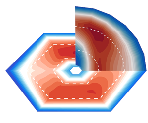
Figure 2 shows contour of the averaged and normalized third-order structure functions for both normal viscous and hyper-viscous cases with various values of  $B_0$. The inertial range is identified with the direction-averaged form of the third-order law, where
  $-3(\overline { Y_l^+}+\overline { Y_l^-})/({8\varepsilon l})$ is beyond a threshold, say 0.9, and marked with the white dashed lines. A straightforward observation is that the isotropic cases at
  $B_0= 0$ present a distribution of the normalized structure functions that is essentially independent of polar angle
  $\theta$. Unlike this isotropic case (
 $B_0=0$), the dark contour lines for
  $B_0=2$ and 5 do not distribute symmetrically. More specifically, the contour lines at small
  $l$ (dark blue regions close to origins) are elongated along the parallel direction
  $\theta =0^\circ$, which can be interpreted as the anisotropy introduced by the mean magnetic field. The contour lines at large
  $l$ (dark blue outer regions) approach a more circular conformation. This is not in conflict with the frequently observed picture of anisotropy in decaying MHD turbulence, as the present system is driven isotropically at large scales. The inertial range exists in the transition region between small and large scales, as marked with the white dashed lines. For non-zero
  $B_0$ cases, the peak value of the normalized third-order structure function at larger
  $\theta$ occurs at smaller scales, which is consistent with the results in Verdini et al. (Reference Verdini, Grappin, Hellinger, Landi and Müller2015) and Wang et al. (Reference Wang, Chhiber, Adhikari, Yang, Bandyopadhyay, Shay, Oughton, Matthaeus and Cuesta2022). The maximum radial transfer rate shifts away from the
  $B_0$ direction at larger
  $B_0$, with the corresponding
  $\theta$ of the maxima for
  $B_0= 2$ and 5 at
  $\theta =0^\circ$ and
  $\theta =30^\circ$, respectively, which is clearer in figure 3.

Figure 2. Comparison of normalized third-order structure functions, i.e. method II in (3.8) with  $-3(\widetilde { Y_l^+}+\widetilde { Y_l^-})/({8\varepsilon l})$ between (a,c,e) simulations with normal viscosity and (b,d,f) simulations with hyper-viscosity with polar angles in the range
  $\theta = [0^\circ :15^\circ :90^\circ ]$. Here,
  $\theta =0^\circ$ represents the parallel direction relative to
  $\boldsymbol {B}_0$, and
  $\theta =90^\circ$ represents the perpendicular direction relative to
  $\boldsymbol {B}_0$. The white dashed lines represent the inertial range, identified with the direction-averaged form of third-order law, i.e. method III in (3.9), where
  $-3(\overline { Y_l^+}+\overline { Y_l^-})/({8\varepsilon l})$ is beyond a threshold, say 0.9. All contours are integrated over
  $\phi$ and time; (a,b)
  $B_0=0$, (c,d)
  $B_0=2$, (e,f)
  $B_0=5$.

Figure 3. Comparison of normalized third-order structure functions, i.e. method II in (3.8) with  $-3(\widetilde { Y_l^+}+\widetilde { Y_l^-})/({8\varepsilon l})$, at
  $B_0=0,2,5$ between (a,c,e) normal viscous and (b,d,f) hyper-viscous simulations with
  $\theta = [0^\circ :15^\circ :90^\circ ]$, and the solid line with triangles represents the direction-averaged profile, i.e. method III in (3.9) with
  $-3(\overline { Y_l^+}+\overline { Y_l^-})/({8\varepsilon l})$. All curves are averaged over
  $\phi$ and time. For non-zero
  $B_0$ the estimated transfer rate peaks at large scales for parallel angles, and at progressively smaller scales for perpendicular angles; (a,b)
  $B_0=0$, (c,d)
  $B_0=2$, (e,f)
  $B_0=5$.
We can see the clear difference between normal and hyper-viscous cases in figure 3, where the normalized third-order structure functions at  $\theta \in [0^\circ :15^\circ :90^\circ ]$ are shown. Also shown is the normalized and direction-averaged third-order structure function, i.e.
  $-3(\overline { Y_l^+}+\overline { Y_l^-})/({8\varepsilon l})$. Even though the normalized third-order structure functions exhibit evident dependence on
  $\theta$, the direction-averaged third-order law attains an accurate cascade rate with less than 5 % error for all cases. The plateau of the direction-averaged form in figure 3 gives a rough idea of the inertial range, which indicates that
  $l\in [0.15,0.43]$ and
  $l\in [0.08,0.55]$ at
  $B_0=0$ can be roughly identified as the inertial range for the normal and hyper-viscous cases, respectively. This elongated inertial range is also consistent with the estimates of the inertial range in figure 1, where
  $k=2{\rm \pi} /l$. Therefore, as expected, hyper-viscosity enables a wider inertial range than normal viscosity and the longer inertial range is beneficial to examine the third-order law.
The hyper-viscous cases show a similar polar angle dependence to the normal viscous cases at low  $B_0$ (i.e. weak anisotropy). At
  $B_0=0$, the individual
  $\theta$ profiles in figure 3 overlap with the direction-averaged profile, indicating the applicability of the 1-D isotropic third-order law. As
  $B_0$ increases, they deviate from the direction-averaged profile. In particular, when
  $B_0$ is large enough (e.g. figure 3(e,f) with
  $B_0=5$), the third-order structure functions for the hyper-viscous cases exhibit distinct peak values from the normal viscous cases. For the normal viscous case, the third-order law tends to underestimate the cascade rate for
  $\theta >45^\circ$, and overestimate the cascade rate for
  $\theta <45^\circ$. As such, the maximum value of the estimated cascade rate is located at
  $\theta =30^\circ$, also shown in figure 2. In contrast, for the hyper-viscous case, the third-order law at
  $\theta \sim 90^\circ$ overestimates the cascade rate and the contour map in figure 2 exhibits two local maxima at
  $\theta =30^\circ$ and
  $\theta =90^\circ$. The maximum at
  $\theta =90^\circ$ could be attributed to the dissipation being concentrated at smaller scales due to hyper-viscosity. As we can see, the energy transfer changes gradually with angles and the most efficient transfer may not necessarily occur in the strictly perpendicular direction.
4.2. Azimuthal angle dependence
In this subsection, the hyper-viscous cases will be used to demonstrate the azimuthal dependence of the third-order structure function. Figure 4(a,c,e) shows the normalized third-order structure function at different  $\theta$ and
  $\phi$. It can be seen that the variability of third-order structure functions in the azimuthal and polar angles increases with the increase of
  $B_0$, indicated by the more scattered distribution of the profiles at higher
  $B_0$. Specifically, at
  $B_0=0$, these individual lines almost collapse, indicating the isotropic features in both the polar and azimuthal directions. At
  $B_0=2$, the peak values of these lines are almost beyond unity. At
  $B_0=5$, the peaks vary beyond and below unity. To further quantify these departures from the actual cascade rates in table 1, figure 4(b,d,f) is plotted by using the peak of each profile, representing the estimated cascade rate. The distribution of these estimates, as marked with the dark circles, is more scattered at a larger
  $B_0$. At
  $B_0 = 2, 5$, the maximum estimated cascade rate can depart from the actual value by 10 % and
  $25\,\%$ and both at
  $\theta =45^\circ$. We expect this departure to be even greater at larger
  $B_0$. From the red line in figure 4(b,d,f), after doing the azimuthal average, the maximum departures from unity reduce to 3 % and 15 % at
  $B_0=2, 5$, respectively.

Figure 4. (a,c,e) Normalized third-order structure functions, i.e. method I in (3.7) with  $-3({ Y_l^+}+ Y_l^-)/({8\varepsilon l})$, for (a,b)
  $B_0=0$, (c,d)
  $B_0=2$ and (e,f)
  $B_0=5$ hyper-viscous cases at different
  $\theta$ and
  $\phi$. Each series of colours represents a fixed
  $\theta$ and varied
  $\phi$, e.g. green lines represent the results at
  $\theta =60^\circ$ and
  $\phi = [0^\circ :60^\circ :300^\circ ]$. (b,d,f) Estimated cascade rates from column (a,c,e) by extracting the peaks of each curve and then normalizing with the total dissipation rate,
  $\varepsilon$. The solid line with circles represents the averaged profile on the azimuthal direction. All curves are time averaged.
Theoretically, given that the number of frames is sufficient to compute a stable average, the averaged structure function should be independent of the azimuthal angles. Therefore, when we describe energy transfer as isotropic in the perpendicular plane we are referring to statistically averaged transfer. When sampling and averaging is limited, e.g. finite snapshots as in direct numerical simulation or directions as in observations are employed, then a residual dependence on the azimuthal directions might persist in the estimates. This dependence could be associated with the locally spatial and temporal fluctuations caused by large-scale structures in the perpendicular plane at large  $B_0$, as observed by Zikanov & Thess (Reference Zikanov and Thess1998). Adequate coverage of azimuthal angles is required to obtain an accurate estimation of cascade rates. To further check the mutual impact of the time and angle averages, the effects of the sampling time will be discussed in the next subsection.
4.3. Effects of time averaging
In this subsection, the hyper-viscous cases will be used to demonstrate the effect of time averaging. At least two aspects of the time averaging are of central importance, one being the time interval (or sampling frequency)  $\Delta T$, and the other being the length of periods
  $T$. We can expect that, in our driven cases, the smaller
  $\Delta T$ and the longer
  $T$, the more reliable the statistics. The time interval
  $\Delta T$ (
 $\Delta T < T_e$, where
  $T_e$ is the large-eddy turnover time) does not show significant impacts on the third-order structure function in our cases (figures are not shown here). Therefore, in the following analysis, we fix
  $\Delta T=0.5T_e$ and focus on the effect of the length of periods
  $T$. These periods are within the statistically stationary periods listed in table 1.
Figure 5 shows the effect of the length of periods (or the number of time frames,  $F$) on the third-order structure function. The third-order law at fixed
  $\theta$ and
  $\phi$ as (3.7), at fixed
  $\theta$ but
  $\phi$ averaged as (3.8) and both
  $\theta$ and
  $\phi$ averaged as (3.9) is shown in the left, middle and right columns, respectively. Three key observations can be made: (i) the direction-averaged profiles require fewer time frames (
 $F$) to converge than the profiles with fixed
  $\theta$ and
  $\phi$. For instance, at
  $B_0= 5$ the direction-averaged profiles converge with 36 time snapshots, while the profiles with fixed
  $\theta$ and
  $\phi$ are not converged until 72 time frames are employed; (ii) a smaller
  $B_0$ requires fewer time frames to converge. The required numbers of time frames for
  $B_0= 0$ and
  $B_0= 5$ to converge are approximately 10 and 70, respectively, without the directional average (figure 5a,d,g). These times are reduced to approximately 5 and 30, respectively, with directional averaging (see figure 5c,f,i); (iii) time averaging is not as effective as the angle coverage, indicated by the different peak values of non-direction-averaged and direction-averaged profiles in the anisotropic cases. Also, by comparing the three columns, the angle averaging makes the plateaus of these plots closer to the actual dissipation rate. For instance, at
  $B_0=5$, the converged profiles without angular averaging, with only azimuthal averaging and with both azimuthal and polar averaging attain peak values of 1.19, 1.09 and 0.98, respectively. This indicates that, compared with the time averaging, the angle averaging is a more effective way to make the calculation of the structure function converge.

Figure 5. Effects of the number of time frames on the calculation of the normalized third-order structure functions at (a–c)  $B_0=0$, (d–f)
  $B_0=2$ and (g–i)
  $B_0=5$ for the hyper-viscous cases. (a,d,g) Method I in (3.7) with fixed
  $\theta = {\rm \pi}/4; \phi = {\rm \pi}/3$. (b,e,h) Method II in (3.8) with fixed
  $\theta = {\rm \pi}/4$ and azimuthal-averaged profiles. (c,f,i) Method III in (3.9) with direction-averaged profiles. Here,
  $T_e$ denotes the large-eddy turnover time at
  $B_0=0$, and
  $F$ represents the number of frames used in the time average. (a,d,g) Fixed
  $\theta = {\rm \pi}/4$ and
  $\phi = {\rm \pi}/3$. (b,e,h) Fixed
  $\theta = {\rm \pi}/4$, Averaging
  $\phi$. (c,f,i) Averaging
  $\theta$ and
  $\phi$.
5. Conclusions
Three-dimensional simulations of incompressible MHD turbulence with normal and hyper-viscosity were conducted with different externally supported (mean) uniform magnetic fields to systematically study the effect of external mean magnetic fields on the cross-scale energy transfer and the third-order law. Three different forms of third-order structure functions were calculated with or without averaging of the azimuthal and polar angles. The results show that, compared with the normal viscous cases, the hyper-viscosity elongates and separates the inertial range from the dissipation range, thus helping the examination of the above-mentioned forms of the third-order law.
The third-order laws governing the behaviour of third-order structure functions in the inertial range are among the few rigorous results about cross-scale energy transfer. Existing studies of energy transfer in the inertial range in MHD and space plasmas have had a particular leaning toward the use of the simplified third-order law under the assumption of isotropy, as implemented in (3.6) (also called the isotropic form). Although the isotropic form is notable in its simplicity and elegance, one should keep in mind that the isotropic assumption is required to arrive at this point. That is, the isotropic form assumes that the energy transfer across scales quantified along one direction is representative of the complex 3-D energy transfer. This inevitably conflicts with the anisotropic nature, especially for solar wind turbulence, which casts doubt on the widespread use of the isotropic form of the third-order law.
To resolve the limitation concerning the isotropic form of the third-order law, we investigate systematically the angular dependence of the energy transfer. As shown by our MHD simulations with varying mean magnetic fields, one can directly recognize that the radial component  $Y_\ell$ of the energy flux
  $\boldsymbol {Y}$ varies systematically over the direction relative to the mean magnetic field (i.e. polar angle
  $\theta$ in spherical coordinates). If we only use the profile along one direction (i.e. choose a polar angle and an azimuthal angle) to represent the energy transfer rate, it could depart significantly from the actual rate, necessitating simultaneous consideration of contributions from different directions to the energy transfer. The strategy developed by Taylor et al. (Reference Taylor, Kurien and Eyink2003) is therefore employed, by which the third-order structure function is computed in many directions and the results are averaged, which is called the direction-averaging method (i.e. method III in (3.9)). We find that the direction-averaged third-order law can predict the energy cascade rates and inertial range accurately, even at very high
  $B_0$, thus providing a convincing scheme for extracting the energy transfer rate in anisotropic flows. The azimuthal angle dependence we find here is counterintuitive, in that the statistics are usually deemed to be statistically isotropic in the plane perpendicular to
  $B_0$. This azimuthal angle dependence was further confirmed with an examination of the number of averaging time frames. More time frames are required to make the calculation of the third-order structure function converge in the anisotropic condition, especially at high
  $B_0$. However, even using enough time frames, the structure function profiles with and without the azimuthal average are still different. We conclude that the time averaging cannot make up for a lack of angle averaging, especially at large values of the mean magnetic field
  $B_0$.
An interesting finding, also seen in earlier studies (Verdini et al. Reference Verdini, Grappin, Hellinger, Landi and Müller2015; Wang et al. Reference Wang, Chhiber, Adhikari, Yang, Bandyopadhyay, Shay, Oughton, Matthaeus and Cuesta2022), is that identified peaks or plateaus of the estimated transfer rate occur at different scales for different angles with respect to the mean magnetic field. Accordingly, this also means that the inertial range will be assigned to different ranges of scales at different angles. Our use of hyper-viscosity produces an extended plateau, facilitating analysis of the inertial range properties. Future studies may find a rationale for understanding how these different ranges come into being, as the balance of local transfer rate competes with dissipation at different angles. Such analyses may require examination of the vector character of the Yaglom energy flux, a subject that we have not engaged in here. It should be noted, however, that there are some studies that have begun such analyses, typically by making assumptions regarding the symmetry of the transfer. Examples include the 2-D (perpendicular) + 1-D (parallel) model employed by MacBride, Smith & Forman (Reference MacBride, Smith and Forman2008), Stawarz et al. (Reference Stawarz, Smith, Vasquez, Forman and MacBride2009) and Stawarz et al. (Reference Stawarz, Smith, Vasquez, Forman and MacBride2010). Such models may require further refinement since at least some prior models enforce the questionable assumption that the transfers of energy in parallel and perpendicular directions are independent.
Funding
We acknowledge the support from NSFC (Grant Nos. 12225204, and 11902138); Department of Science and Technology of Guangdong Province (Grant Nos. 2019B21203001 and 2020B1212030001); the Shenzhen Science and Technology Program (Grant No. KQTD20180411143441009). Y.Y. and W.H.M. are supported by NSF grant AGS02108834 and by NASA under the IMAP project at Princeton (subcontract 0000317 to Delaware). W.H.M. is also supported as a Co-Investigator on the Helioswarm project. The assistance of resources and services from the Center for Computational Science and Engineering of Southern University of Science and Technology is also acknowledged.
Declaration of interests
The authors report no conflict of interest.
Appendix
To choose the hyper-viscosity coefficient ( $\nu _h$) and order (
 $h$), three different orders of hyper-viscosity (
 $h$) with 256
 $^3$ grids are tested, as shown in figure 6. We tuned the coefficient (
 $\nu _h$) to ensure all these 3 test cases with
  $k_{max} \eta _{k,v} \sim 1.5$ to achieve a long inertial range while resolving the dissipation range. It shows that the higher order (
 $h=3$) of hyper-viscosity can further extend the inertial range, while the bottleneck effect is more obvious, as shown in the compensated energy spectra, consistent with Frisch et al. (Reference Frisch, Kurien, Pandit, Pauls, Ray, Wirth and Zhu2008). Following these tests we decided that the choice of
  $h=2$ performs very well for our purposes.

Figure 6. Comparison of the normal ( $h=1$) and hyper-viscous (
 $h=2, 3$) cases at
  $B_0=0$ with 256
 $^3$ grids. (a) Compensated energy spectra; (b) energy transfer rate.
To further evaluate the bottleneck effect, we also compared the choice of the hyper-viscosity coefficients with 512 $^3$ grids at
  $h=2$, as shown in figure 7. Both the energy spectra and structure function profiles show that the present hyper-viscosity with
  $\nu _h=2\times 10^{-7}$ and
  $k_{max} \eta _{k,v}=1.73$ achieve the longer inertial range, compared with the larger
  $\nu _h$ at
  $8\times 10^{-7}$ with
  $k_{max} \eta _{k,v}=2.47$. Furthermore, from the structure function profiles, this bottleneck effect is indeed not visible as per Biskamp & Müller (Reference Biskamp and Müller2000).

Figure 7. Comparison of the hyper-viscous ( $h=2$) cases with different viscosity coefficients at
  $B_0=0$ with 512
 $^3$ grids. (a) Energy spectra; (b) third-order structure function.


