


Motivation and hypothetical model for hydrocarbons on Mars
We discovered a correlation between the aligned (combed) gravity strike angles, based on the global gravity field models, and known oil and gas deposit locations in the Caspian Sea and in Ghawar, Saudi Arabia (see Klokočník and Kostelecký, Reference Klokočník and Kostelecký2014). Later, we extrapolated to possible oil and gas sources in diverse areas on the Earth (Klokočník et al., Reference Klokočník, Kostelecký, Bezděk, Cílek, Kletetschka and Staňková2020c, Reference Klokočník, Kostelecký, Bezděk and Cílek2021b) and to groundwater on the Moon (Kletetschka et al., Reference Kletetschka, Klokočník, Hasson, Kostelecký, Bezděk and Karimi2022). It is logical to extend this method to Mars because after the Earth and the Moon, we now have sufficient knowledge about the gravity field of Mars. Finding hydrocarbons on Mars would mean finding indication for a form of past life on Mars.
The idea of hydrocarbons on Mars is not a new one. Thiophenes, formed at the bottom of a hypothetical ancient Martian freshwater lake (Gale Crater), found by Curiosity, could be markers of life on Mars (Science 2013; Heinz and Schulze-Makuch, Reference Heinz and Schulze-Makuch2020). [Thiophenes contain four carbon atoms and one sulphur atom; they occur in kerogens, bitumen, coals, crude oil (petroleum), sediments (ibid., p. 552) and white truffles (mushrooms).] The rover of Perseverance found evidence for ancient hot magma, impact melt or volcanic deposit, variably altered to carbonate and water (e.g. Farley et al., Reference Farley, Stack, Shuster, Horgan, Hurowitz, Tarnas, Simon, Sun, Scheller, Moore, McLennan, Vasconcelos, Wiens, Treiman, Mayhew, Beyssac, Kizovski, Tosca, Williford, Crumpler, Beegle, Bell, Ehlmann, Liu, Maki, Schmidt, Allwood, Amundsen, Bhartia, Bosak, Brown, Clark, Cousin, Forni, Gabriel, Goreva, Gupta, Hamran, Herd, Hickman-Lewis, Johnson, Kah, Kelemen, Kinch, Mandon, Mangold, Quantin-Nataf, Rice, Russell, Sharma, Siljeström, Steele, Sullivan, Wadhwa, Weiss, Williams, Wogsland, Willis, Acosta-Maeda, Beck, Benzerara, Bernard, Burton, Cardarelli, Chide, Clavé, Cloutis, Cohen, Czaja, Debaille, Dehouck, Fairén, Flannery, Fleron, Fouchet, Frydenvang, Garczynski, Gibbons, Hausrath, Hayes, Henneke, Jorgensen, Kelly, Lasue, Le Mouélic, Madariaga, Maurice, Merusi, Meslin, Milkovich, Million, Moeller, Núnez, Ollila, Paar, Paige, Pedersen, Pilleri, Pilorget, Pinet, Rice, Royer, Sautter, Schulte, Sephton, Sharma, Sholes, Spanovich, St. Clair, Tate, Uckert, VanBommel, Yanchilina and Zorzano2022). River deltas are potentially preserving carbon-containing organic compounds. The Earth's river and fossil deltas, such as the Nile, Niger and Mississippi, represent some of the most suitable places for the origin of petroleum deposits, because the rivers are carrying biogenic elements (P, Fe, V and others), released from weathered rocks. The organic detritus is quickly buried by eroded sediments to the depths suitable for oil genesis (e.g. Hunt, Reference Hunt1996; Montmessin et al., Reference Montmessin, Smith, Langevin, Mellon and Fedorova2017).
These and other findings, independent of our novel approach (based on global gravity aspects) provided a clear motivation for us to investigate this topic, having already had some experience with the Earth. Here we present our first results.
We start with the following hypothesis. Just as life arose very quickly on the Earth after the cooling of the Earth's crust and the world's oceans (Mojzsis et al., Reference Mojzsis and Arrhenius1998; Altermann, Reference Altermann and Seckbach2007), an aquatic environment suitable for the evolution of life existed on Mars for a sufficiently long time (Baker, Reference Baker2001; Ehlmann et al., Reference Ehlmann, JF, SL, J-P, Meunier, AA and Langevin2011). However, the magnetic field of Mars was weaker than that of the Earth and the atmosphere lacked the protection of the ozone layer, so we consider submarine hot springs to be the most likely ‘oases’ where life originated (Abramov and Mojzsis, Reference Abramov and Mojzsis2009). These, as a result of strong volcanism and meteoritic impacts, probably existed for a sufficiently long time (Rossi et al., Reference Rossi, Neukum, Pondrelli, van Gasselt, Zegers, Hauber, Chicarro and Foing2008) for the evolution of life, e.g. in the form of biofilms and microbial coatings (Blumenberg, Reference Blumenberg, Kile and Tyler2010; Seckbach and Chela-Flores, Reference Seckbach and Chela-Flores2012).
The most likely type of life on Mars, like on the Earth, was anaerobic chemotrophs probably tied to vicinity of warm underwater springs (Westall et al., Reference Westall, Foucher, Bost, Bertrand, Loizeau, Vago, Kminek, Gaboyer, Campbell, Bréhéret, Gautret and Cockell2015). We hypothesize that these organic remains were redistributed by later processes such as pressure and temperature changes, resulting from sediment burial, and may appear as biosignatures or chemofossils in suitable locations that may be analogous to terrestrial oil traps.
The earliest morphological manifestations of life are tied to simple shapes that can arise both organically and inorganically, e.g. during the coralloid growth of crystalline aggregates in aqueous glass or silicate colloids. This is one of the reasons for the long discussion concerning, e.g. the findings of real or apparent microbes from the Australian Apex Chert and other sites (Brasier et al., Reference Brasier, Green, Lindsay, McLoughlin, Jephcoat, Kleppe, Steele and Stoakes2005; Schopf, Reference Schopf2006), despite the sites being relatively easy to reach and sample, at least in comparison with Mars.
In search of the earliest terrestrial life, we often focus on the geochemical remains of life – on chemofossils with characteristic isotope compositions mainly of carbon and sulphur, and the abundance of organic compounds and trace elements. But this yields ambiguous rather than probabilistic results (Blumenberg, Reference Blumenberg, Kile and Tyler2010). Terrestrial crude oil can be viewed as both biologically and catalytically pressure- and temperature-processed chemofossils (in the presence of iron and manganese oxides). Unlike many other remnants of organic life that remain more or less ‘in situ’ in the rock mass, petroleum usually has a long dynamic and migratory history. The basic mechanism of oil reservoir formation is the transport of oil droplets in a water emulsion, the gravitational separation of lighter liquid and gaseous hydrocarbons, and their deposition in oil traps. This is mostly an impermeable, anticlinal structure that morphologically resembles an umbrella (Hunt, Reference Hunt1996).
Extensive fluid migration occurred on Mars at the end of the Noachian (ca. 4.5–3.5 Ga) and during the Hesperian (ca. 3.5–2.5 Ga). During this long period, water on Mars either moved by gravity, retreated into drying basins or underwent hydrothermal circulation (Zurek, Reference Zurek, Tolson, Bougher, Lugo, Baird, Bell and Jakosky2017). Good evidence for the existence of large hydrothermal systems comprises, for example, ridges linked to linear tectonic structures (see the figure of Candor Chasma in Vogt, Reference Vogt2008, p. 36). They resemble silicified areas commonly found on the Earth along faults. We guess that on Mars, with its huge volcanoes and voluminous lava outpourings, we have to expect the existence of large hydrothermal systems and thus water flows, including possible hydrocarbons (for the Earth analogue, see Van Kranendonk, Reference Van Kranendonk2006). This is a situation commonly addressed by terrestrial petroleum geology.
The question of petroleum traps on Mars is highly problematic because most strata, as shown by images of the Martian landscape, are deposited horizontally or slightly tilted. However, the alternation of layers indicates, in some cases, regular environmental changes as well as the possibility of deposition of insulating clay layers of, e.g. aeolian origin (Kramer et al., Reference Kramer, Potter, Marais and Peterson2003; Kite et al., Reference Kite, Rafkin, Michaels, Dietrich and Manga2011). A similar situation between the arrangement of strike angles and the more frequent occurrence of oil (as a specific type of chemofossil) is expected on Mars.
It is important to note at the outset of this paper that the gravity aspects (and specifically the strike angles) provide three types of mutually overlapping information:
(1) Information about geological structure. In evaluating terrestrial analogies, large-scale, uniform structures little affected by fault tectonics turn out to be important. On Mars, large-scale deltas, outwash cones and possible lahars would probably best suit these conditions.
(2) Information on water circulation. The amount of water as a medium carrying petroleum emulsions is many times greater than the hydrocarbons themselves. Therefore, ‘ordered’ (aligned, combed) strike angle formations are more likely to give information about the groundwater flows than about oil/gas. Again, based on terrestrial analogies, we assume that they mainly indicate the areas with uniform linear flows.
(3) Occurrence of hydrocarbons. This case is mainly due to both of these factors, but also due to the existence of source rocks and their porosity.
In recent years, we have been analysing the gravity aspects (Kalvoda et al., Reference Kalvoda, Klokočník, Kostelecký and Bezděk2013; Klokočník and Kostelecký Reference Klokočník and Kostelecký2014), especially the strike angles, around major oil/gas fields such as Ghawar, the Caspian Sea, and the Middle East. For the fields, but also for the areas where groundwater reservoirs exist (additional to or in combination with hydrocarbons), a combed structure with a parallel course of strike angles is typical (Klokočník et al., Reference Klokočník, Kostelecký and Bezděk2017a, Reference Klokočník, Kostelecký, Cílek, Bezděk and Pešek2017b, Reference Klokočník, Kostelecký, Cílek, Bezděk and Pešek2018, Reference Klokočník, Kostelecký and Cílek2020a, Reference Klokočník, Kostelecký, Bezděk and Cílek2021b, Reference Klokočnik, Bezděk, Kostelecky, Foulger, Hamilton, Jurdy, Stein, Howard and Stein2022b). These structures on the Earth indicate places where underground reservoirs or oil traps are not disturbed by later folding or fault tectonics. The same methodology also succeeded in a search for groundwater for the Artemis mission near the southern pole of the Moon (Kletetschka et al., Reference Kletetschka, Klokočník, Hasson, Kostelecký, Bezděk and Karimi2022). Now we ‘expand’ to Mars, having at our disposal, not only wishful thinking, but also the data from quality satellite measurements.
People often transfer directly our knowledge valid for the Earth to the other, at least partly similar celestial bodies, but it may have some obstacles. On the one hand, the size of the body is important, and in turn, the local geology differs. For example, because the Moon is small, bending stresses are fully capable of supporting topographic loads up to long-wavelengths (expressed by low degree/order harmonics in the spherical expansion of the disturbing potential, see below) and this will naturally affect how the gravity field is expressed. For that reason, the geological features on the Earth, the Moon and Mars will have different form of gravitational expressions just due to planetary size. On the other, gravitation, as it is, is universal: crater/basin/fault/volcano/lake, etc. have generally common signal in terms of the gravity aspects everywhere (many examples are provided in our Supplements 2 and 3). We can and we will transfer but with caution and under control of geologists.
From the viewpoint of a geologist: what are the possibilities of comparing the gravimetric record on Earth, Moon and Mars, which have a different geological evolution? Some features are very similar to each other, as geomorphology shows – in particular volcanic formations, including secondary deformations such as slope movements and lahars. The steep walls of impact craters are very often subject to slope deformation and landslides, as we know from Earth. The very important analogy is the filling of linear depressions and valleys, where, for example, the old Nile valleys beneath the aeolian sediments of the Sahara have gravimetric characteristics similar to river valleys on Mars. The record of flat-lying sedimentary basins is analogous. In contrast, the record of impact processes is largely different. If mascons existed on Earth, they were reworked by plate tectonics, and likewise most large terrestrial impact craters were heavily altered by erosion, which denuded several kilometres of rock, especially in Precambrian terrains.
Our procedure is not able to precisely determine the locations of possible hydrocarbons on Mars, but could serve as a refinement criterion for further research; in other words, as an additional pre-drilling constraint, an indicator, ‘conditioner’ or information that the probability of the presence of oil/gas/water deposits in the area is high or low. This remote-sensing tool is cheap.
Introduction
Water (H2O) on Mars exists as water ice, e.g. in the large, thick northern Martian polar cap. It can also be expected to lie under the surface frozen to ground-ice (permafrost), theoretically everywhere (Feldman, Reference Feldman, Mellon, Maurice, Prettyman, Carey, Vaniman, Bish, Fialips, Chipera, Kargel, Elphic, Funsten, Lawrence and Tokar2004). Minerals on Mars revealed that Mars had and may have water in Meridiani Planum (e.g. Herkenhoff et al., Reference Herkenhoff, Squyres, Arvidson, Bass, Bell, Bertelsen, Ehlmann, Farrand, Gaddis, Greeley, Grotzinger, Hayes, Hviid, Johnson, Jolliff, Kinch, Knoll, Madsen, Maki, McLennan, McSween, Ming, Rice, Richter, Sims, Smith, Soderblom, Spanovich, Sullivan, Thompson, Wdowiak, Weitz and Whelley2004; Klingelhöfer et al., Reference Klingelhöfer, Morris, Bernhardt, Schröder, Rodionov, de Souza, Yen, Gellert, Evlanov, Zubkov, Foh, Bonnes, Kankeleit, Gütlich, Ming, Renz, Wdowiak, Squyres and Arvidson2004; Squyres et al., Reference Squyres, Grotzinger, Arvidson, Bell, Calvin, Christensen, Clark, Crisp, Farrand, Herkenhoff, Johnson, Klingelhöfer, Knoll, McLennan, McSween, Morris, Rice, Rieder and Soderblom2004) [φ = 0°N, λ = 2°W]. ‘Fluvial’ features were found all over the cratered plateau of the Southern Hemisphere (Forget et al., Reference Forget, Costard and Lognonné2008), already based on Mariner 9 observation, and recently elsewhere by Perseverance (Farley et al., Reference Farley, Stack, Shuster, Horgan, Hurowitz, Tarnas, Simon, Sun, Scheller, Moore, McLennan, Vasconcelos, Wiens, Treiman, Mayhew, Beyssac, Kizovski, Tosca, Williford, Crumpler, Beegle, Bell, Ehlmann, Liu, Maki, Schmidt, Allwood, Amundsen, Bhartia, Bosak, Brown, Clark, Cousin, Forni, Gabriel, Goreva, Gupta, Hamran, Herd, Hickman-Lewis, Johnson, Kah, Kelemen, Kinch, Mandon, Mangold, Quantin-Nataf, Rice, Russell, Sharma, Siljeström, Steele, Sullivan, Wadhwa, Weiss, Williams, Wogsland, Willis, Acosta-Maeda, Beck, Benzerara, Bernard, Burton, Cardarelli, Chide, Clavé, Cloutis, Cohen, Czaja, Debaille, Dehouck, Fairén, Flannery, Fleron, Fouchet, Frydenvang, Garczynski, Gibbons, Hausrath, Hayes, Henneke, Jorgensen, Kelly, Lasue, Le Mouélic, Madariaga, Maurice, Merusi, Meslin, Milkovich, Million, Moeller, Núnez, Ollila, Paar, Paige, Pedersen, Pilleri, Pilorget, Pinet, Rice, Royer, Sautter, Schulte, Sephton, Sharma, Sholes, Spanovich, St. Clair, Tate, Uckert, VanBommel, Yanchilina and Zorzano2022). It can be groundwater or it can be due to hydrothermal circulation. Opportunity confirmed the presence of haematite, tracks of water in hydrated sulphate salts. Spirit at Gusev crater (probably a former lake) [14.7S, 175.5E], proved there were sedimentary deposits, haematite, sulphate salts, oxidized iron or goethite that cannot be formed without water (Forget et al., Reference Forget, Costard and Lognonné2008). Near the Isidis basin, magnesium carbonate was found by the MRO; this indicates non-acid water with favourable conditions for the evolution of life (Murchie et al., Reference Murchie, Mustard, Ehlmann, Milliken, Bishop, McKeown, Noe Dobrea, Seelos, Buczkowski, Wiseman, Arvidson, Wray, Swayze, Clark, Des Marais, McEwen and Bibring2009). Groundwater was assessed in Utopia Planitia using the Shallow Radar Instrument on the MRO; 2013; NASA/JPL-Caltech/Univ. of Rome/ASI/PSI. Recently, the Zhurong rover of China's Tianwen-1 mission, which landed in southern Utopia Planitia, identified hydrated sulphate/silica materials on the Amazonian terrain at the landing site (Liu et al., Reference Liu, Wu, Zhao, Pan, Wang, Liu, Zhao, Zhou, Zhang, Wu, Wan and Zou2022).
The lahars (e.g. Pedersen Reference Pedersen2013), probably occurring in many places on Mars (more in Sections ‘Strike angles’ map documentation’ and ‘Summary of our observations and discussion’), are connected with volcanoes and water. Under Martian conditions, a significant amount of water generating the lahars is still present as ice in the lahar deposits, e.g. near Elysium Mons (Pedersen, Reference Pedersen2013). The necessary condition for the formation of lahars on Mars is the existence of hot volcanic sediments, falling on the frozen ground that may release water.
One characteristic of rocks formed by flowing water is fine, undulating layers of sediment (crossbeds). Several rocky surfaces revealed small laminations indicating layering that may have been formed by gently flowing water (e.g. Edgar et al., Reference Edgar, Grotzinger, Bell and Hurowitz2014; McCollom, Reference McCollom2018). Traces of water interaction were discovered at Gusev crater/Columbia Hills at northern Martian palaeo-ocean (NMPO) (Mittlefehldt et al., Reference Mittlefehldt, Gellert, vanBommel, Ming, Yen, Clark, Morris, Schröder, Crumpler, Grant, Jolliff, Arvidson, Farrand, Herkenhoff, Bell, Cohen, Klingelhöfer, Schrader and Rice2018) and elsewhere (Mittlefehldt et al., Reference Mittlefehldt, Gellert, vanBommel, Ming, Yen, Clark, Morris, Schröder, Crumpler, Grant, Jolliff, Arvidson, Farrand, Herkenhoff, Bell, Cohen, Klingelhöfer, Schrader and Rice2018; Orosei et al., Reference Orosei, Lauro, Pettinelli, Cicchetti, Coradini, Cosciotti, Di Paolo, Flamini, Mattei, Pajola, Soldovieri, Cartacci, Cassenti, Frigeri, Giuppi, Martufi, Masdea, Mitri, Nenna, Noschese, Restano and Seu2018; Galofre et al., Reference Galofre, Jellinek and Osinski2020; McCollom and Hynek, Reference McCollom and Hynek2021). Lauro et al. (Reference Lauro, Pettinelli, Caprarelli, Guallini, Rossi, Mattei, Cosciotti, Cicchetti, Soldovieri, Cartacci, Di Paolo, Noschese and Orosei2021) announced there was liquid water, with the discovery of subsurface water ice lakes under Mars' southern ice cap.
Geomorphologic evidences for water on Mars from orbiters as well as landers and rovers (from Mariner 9 to Perseverance) are numerous and diverse (see also the text below about the palaeo-ocean), like carved valleys, graben, rifts, eroded grooves, branched streams, streambeds, floods, deltas, channels probably associated with melting ice deposits, lake basins, thick deposits, perhaps gully deposits, lahars, possible groundwater springs or ancient groundwater structures. The presence and size of Martian channels provide the most compelling evidence for the existence of a hydrologic cycle and large amounts of water on Mars (more below).
Palaeo-ocean
The existence of a primordial ocean of liquid water has been predicted by Brandenburg (Reference Brandenburg1987), repeatedly proposed and challenged and is still discussed (e.g. Baker et al., Reference Baker, Strom, Gulick, Kargel and Komatsu1991; Parker et al., Reference Parker, Gorsline, Saunders, Pieri and Schneeberger1993; Head et al., Reference Head, Hiesinger, Ivanov, Kreslavsky, Pratt and Thomson1999; Clifford and Parker, Reference Clifford and Parker2001; Frey et al., Reference Frey, Roark, Shockey, Frey and Sakimoto2002; Buczkowski and McGill, Reference Buczkowski and McGill2003; Ghatan and Zimbelman, Reference Ghatan and Zimbelman2006; Forget et al., Reference Forget, Costard and Lognonné2008; Di Achille and Hynek, Reference Di Achille and Hynek2010; Zuber, Reference Zuber2018 and further references in this paper; Nazari-Sharabian et al., Reference Nazari-Sharabian, Aghababaei, Karakouzian and Karami2020).
The general consensus is that the northern regions of Mars were covered by an ocean. Finding one particular coastline, however, is problematic. The ocean on Mars probably existed in some form for at least 1 billion years, and it is logical that during this time its level must have changed several times, especially during the later drying phase. Carr and Head (Reference Carr and Head2003) analysed earlier shorelines and concluded that in many cases these were lithological boundaries, mainly lava flow margins, rather than oceanic shorelines. The earliest shorelines have probably been destroyed or modified by extensive sheet erosion (Irwin et al., Reference Irwin, Maxwell, Howard, Craddock and Leverington2002). Among the many levels of former ocean surfaces, it is most important to find the most long-term level that indicates stable conditions that may have led to the origin and evolution of life (Section ‘Extent of the palaeo-ocean’). With the gravity data alone, we cannot speak about age.
The main evidence that Mars once had oceans remains the presence of potential shorelines (see already Parker et al., Reference Parker, Gorsline, Saunders, Pieri and Schneeberger1993), although they may have undergone changes due to various reasons (e.g. Citron et al., Reference Citron, Manga and Hemingway2018a, Reference Citron, Manga and Tan2018b). This shoreline in general separates the topographically higher southern part (highlands) from the northern lowlands (topographic depression). Further arguments for the palaeo-ocean are the chemical properties of the Martian soil and atmosphere (e.g. Villanueva et al., Reference Villanueva, Mumma, Novak, Käufl, Hartogh, Encrenaz, Tokunaga, Khayat and Smith2015), and formatting valley networks linked to the volcanism of Tharsis or the roughness of the terrain or its dielectric properties (for more references, see Zuber, Reference Zuber2018).
All of this was inspiring for the development of our own view about the palaeo-ocean based on the gravity aspects and topography computed using the latest gravity field models, surface topography data and magnetic data (Klokočník et al., Reference Klokočník, Kletetschka, Kostelecký, Bezděk and Karimi2022c, Reference Klokočník, Kletetschka, Kostelecký and Bezděk2023). More about this topic is provided in Section ‘Extent of the palaeo-ocean’.
Water is also likely to be contained in the so-called ‘fretted terrain’ near the dichotomy boundary between the northern lowlands and southern highlands. It was discovered as a group of salty lakes hidden beneath the surface and as river deltas (e.g. Haberle et al., Reference Haberle, Clancy, Forget, Smith and Zurek2017).
Liquid water is consistent with warm and wet early Mars for a sufficient time. An alternative hypothesis has been formulated by Burt (Reference Burt2022). He claims that Spirit, Opportunity and Curiosity observations of layered sediments ‘…appear to be inconsistent with published assumptions involving deposition by liquid water…’. He explains the observations by ‘…rapid sediment deposition during Late Noachian impact bombardment followed by local hydration and alternation of sediment by surficial acid condensates…’.
Organic traces
The landers Sojourner (1997), Opportunity (2004–2018), Spirit (2004–2010), Curiosity (2012–), InSight (2018–), Perseverance (2021–) and China's Tianwen-1 (2022–) discovered indications for subterranean life on Mars. [The landing sites of Martian missions are shown in Supplementary material S3 (Fig. S3: 2), that of Perseverance also in Fig. 8(e).]
Plankton and algae, proteins and the life that's floating in the seas, as they die, fall to the bottom; these components will be one of the sources of oil and gas. Spirit and Opportunity found evidence for the past wet conditions on Mars (majority opinion) that could have supported microbial life (fossils of bacteria, stromatolites), see, e.g. Forget et al. (Reference Forget, Haberle, Montmessin, Levrard and Head2006). The Perseverance rover was sent primarily to search for signs of life (e.g. Witze, Reference Witze2022); it landed in ‘Jezero (Lake) crater’ (Isidis), φ = 18.447°N and λ = 77.402°E, close to the dichotomy boundary, in proximity to the hypothetical NMPO. The reason for this choice is that scientists think this might have been one of the ancient lakes fed by Martian rivers. Parts of the Jezero may be rich in carbonates. ‘…If Mars contains substantial subsurface life, the most detectable signature of this life on the Martian surface would be gases generated by the life percolating up to the surface and venting into the Martian atmosphere…’, claims McGovan (Reference McGovan2020). Thiophenes found in dried-up mud on Mars (Heinz and Schulze-Makuch, Reference Heinz and Schulze-Makuch2020) could be a sign of past life.
Do not forget the external sources of organic components, we recall Nakano et al. (Reference Nakano, Hirakawa, Matsubara, Yamashita, Okuchi, Asahina, Tanaka, Suzuki, Naraoka, Takano, Tachibana, Hama, Oba, Kimura, Watanabe and Kouchi2020) indicating that larger organics are present in meteorites than previously thought. They wrote: ‘…we experimentally demonstrate that abundant water and oil are formed via the heating of a precometary-organic-matter … This implies that H2O ice is not required as the sole source of water on planetary bodies … study also suggests that petroleum was present in the asteroids…’.
However, to cool our optimism, it is good to note that most organic molecules are prebiotic: formed through inorganic chemical processes everywhere in space (well known to astronomers). Organic traces do not automatically mean traces of life (e.g. Chela-Flores, Reference Chela-Flores2019).
Considerations about hydrocarbons
Nearly all coal, oil and sedimentary source rocks associated with coal, oil and natural gas on the Earth contain molecules of biological origin (according to conventional theory). Mars may contain subsurface deposits of oil and natural gas indicating past life. Reservoir source rocks are porous and absorbent, and can be saturated with water, oil and gas in various combinations. They should thus provide contrasting (higher) porosity, and relatively lower density, with the relevant changes in the gravity signal in a form of the gravity aspects as they are known for lower density causative bodies in various places on the Earth (depending on the background beneath the sedimentary layers). This is at the core of our remote-sensing approach with global gravity data.
We are, however, well aware of the non-uniqueness of gravity modelling for decoding sources of ground density variations and thus other data (magnetic, seismic, topographic) are always welcome and used if available – here it is surface topography from the MGS MOLA altimeter (Mars Global Surveyor, Mars Orbiter Laser Altimeter) and magnetic intensities from proxies (Connerney et al., Reference Connerney, Acuna, Ness, Kletetschka, Mitchell, Lin and Reme2005; Langlais et al., Reference Langlais, Thébault, Houliez, Purucker and Lillis2019).
Overview
We note first of all the data used (Section ‘Gravity and topography data and reference ellipsoid’) and our method (Section ‘Method’), and then, we describe our preparatory truncation tests (Section ‘Preparatory truncation tests’) to increase confidence and credibility that we are studying real features and not artefacts. Further on, we present global results (Section ‘Strike angles globally’), regional results for the polar caps (Section ‘Strike angles for the polar areas’) and results for the individual zones of the hypothetical palaeo-ocean (Section ‘Individual zones/segments in the palaeo-ocean’) – its extent on the planet is estimated in Section ‘Extent of the palaeo-ocean’. The basic question is where do we look for organic compounds or hydrocarbons bearing deposits? We suggest criteria for this in Section ‘Criteria’ and apply them in Section ‘Strike angles’ map documentation’. Discussion is presented in Section ‘Summary of our observations and discussion’ and conclusions in the final section. We also have three supplements: S1 for theory, S2 with tutorial tests and S3 containing the main results (many more figures than can be included in the main text).
Gravity and topography data and reference ellipsoid
As an input to all of our analyses, we make use of the gravity field models in terms of spherical harmonic expansion (Stokes parameters). For Mars, we use model NASA JPL JGMRO_120F (Konopliv et al., Reference Konopliv, Park Ryan, Rivoldini, Baland, Le Maistre and Van Hoolst2020) to degrees and orders (d/o) = 80. The corresponding ground resolution is about 130 km or ~2.5°. This is much less compared to the Earth and the Moon (about 10 km in both cases) and means a partial hindrance for interpretations. One must be cautious. On the contrary, it is much better than our present knowledge of the gravity field of Venus or Mercury.
The surface topography data come from the altimeter MOLA on board the MGS (Lemoine et al., Reference Lemoine, Smith, Rowlands, Zuber, Neumann, Chinn and Pavlis2001; Smith et al., Reference Smith, Zuber, Frey, Garvin, Head, Muhleman, Pettengill, Phillips, Solomon, Zwally, Banerdt, Duxbury, Golombek, Lemoine, Neumann, Rowlands, Aharonson, Ford, Ivanov, Johnson, McGovern, Abshire, Afzal and Sun2001). The MOLA is linked to the gravity model, fixed areocentrically. The total elevation uncertainty is ‘at least 3 m’ (Lemoine et al., Reference Lemoine, Smith, Rowlands, Zuber, Neumann, Chinn and Pavlis2001); we take 10 m. The topography from the MOLA in this study is given in the ground (horizontal) resolution of 0.25°.
We work with planetographic (ellipsoidal, areographic, areodetic) latitude – analogous to geodetic (not geocentric) latitude on the Earth, related to the reference rotational ellipsoid; the adopted semimajor axis of the reference ellipsoid: a = 3396.19 km, the polar flattening ratio: 1/flattening =169.8. Smith et al. (Reference Smith, Zuber, Frey, Garvin, Head, Muhleman, Pettengill, Phillips, Solomon, Zwally, Banerdt, Duxbury, Golombek, Lemoine, Neumann, Rowlands, Aharonson, Ford, Ivanov, Johnson, McGovern, Abshire, Afzal and Sun2001) wrote that the MOLA team provided planetocentric (areocentric) coordinates, thus a transformation was needed, because the difference in both types of latitudes can be significant at small to medium scales. It is not, however, in our case – we have global and large-scale views.
Further on, we will speak simply about ‘latitudes’ θ and ‘longitudes’ λ. We count them from 0 to 180° to the east and from 0 to −180° to the west or from 0 to 360° to the east. The choice of zero longitude (prime meridian) has been made by astronomers and it is de facto arbitrary. Mariner 9 provided extensive imagery of Mars in 1972 and a small crater Airy-0 in Sinus Meridiani (Arabia Terra) was chosen for the definition of 0.00° longitude (by the IAU, the definition is still valid).
For more information about Data for Mars, see Section ‘Preparatory truncation tests’ (truncation tests). To perform the truncation tests for the Earth and the Moon, as a ‘tutorial’ for Mars, we used EIGEN 6C4 to d/o = 2190 (Förste et al., Reference Förste, Bruinsma, Abrikosov, Lemoine, Schaller, Goetze, Ebbing, Marty, Flechtner, Balmino and Biancale2014) and GRGM1200A to d/o = 600 (Lemoine et al., Reference Lemoine, Goossens, Sabaka, Nicholas, Mazarico, Rowlands, Loomis, Chinn, Neumann, Smith and Zuber2014), respectively.
Method
We work with gravity aspects. Theory of the gravity aspects (descriptors) comes from Pedersen and Rasmussen (Reference Pedersen and Rasmussen1990), Beiki and Pedersen (Reference Beiki and Pedersen2010) and Kalvoda et al. (Reference Kalvoda, Klokočník, Kostelecký and Bezděk2013); it is summarized in our two books (Klokočník et al., Reference Klokočník, Kostelecký and Bezděk2017a, Reference Klokočník, Kostelecký and Cílek2020a) and also in Supplementary material S1. Instead of the traditional gravity anomaly alone, we work with a set of functions of disturbing gravity potential (which is represented by a global gravity field model in terms of harmonic geopotential coefficients – Stokes parameters). This set of gravity aspects contains: (i) the gravity anomaly (or disturbance) Δg, (ii) the Marussi tensor (Γ) of the second derivatives of the disturbing potential (Tij), with the second radial component Tzz, (iii) two of just three gravity invariants (Ij), (iv) their specific ratio (I), (v) the strike angles (θ) and (vi) the virtual deformations (vd).
The gravity aspects are sensitive in various ways to the underground lithological density contrasts (variations) and stress field orientation due to causative bodies. They provide – as a group – much more complete, detailed, in-depth and thorough information about the ground density variations. The set of gravity aspects informs about the location, shape, orientation, tendency towards two-dimensional (2D) or three-dimensional (3D) patterns, stress tendencies and about tensions, although the input data are always the same – the geopotential coefficients of a static gravity field model.
Here, we mostly need the strike angle (Supplement S2). Geophysically, the strike angles θ show directions that are important for a description of the ground structures; they may indicate areas with a lower porosity or a ‘stress direction’ or both. They provide evidence about the anisotropy, e.g. about the target material in the case of impact features. The strike angles seem to be parallel to the weakness in the strength of the rock, e.g. the direction schistosity and/or presence of micro-faults.
It is a usual situation that the strike angle θ has diverse directions, as projected on the Earth's surface (see the tutorial part of S2, Fig. S2: 3). The combed strike angles are θ oriented specifically in the given (studied) area (Fig. S2: 3–15). The alignments have various forms: (1) linear, roughly in one and the same direction (e.g. Fig. S2: 5–9), typical for valleys, trenches, faults and catenae, or (2) creating a halo around circular features, the impact craters and basins (Fig. S2: 3, 4, 10–13) or (3) creating ‘plates’ ( = blocks) with the same orientation inside one plate and a different orientation of θ among the plates (e.g. Fig. S2: 6–9, 13–15). It is not so important which direction of θ the plate is in, what is important is the unidirectionality (and its large extent).
Theory and statistics for the combed θ may have various forms, see, e.g. Klokočník et al. (Reference Klokočník, Kostelecký and Bezděk2019) or Kletetschka et al. (Reference Kletetschka, Klokočník, Hasson, Kostelecký, Bezděk and Karimi2022); see also tutorial training in Fig. S2: 16–20. Here, we follow Kletetschka et al. (Reference Kletetschka, Klokočník, Hasson, Kostelecký, Bezděk and Karimi2022). For the point P in question, we select points Bi around P. The ‘comb coefficient’ in P is then equal to the weighted mean value of the scalar product of the unit vector in P with the unit vectors in Bi. The Comb factor is always in the interval <0, 1>. For perfectly aligned (combed, correlated, parallel) vectors from the given surroundings of the point P, we have Comb = 1. The scalar product (cosine) is ‘flat’ around zero, thus Comb ≥ 0.99 for a very good correlation.
The gravity aspects alone cannot determine the locations or areas where hydrocarbons or any other remnants of life on Mars can be found, but they can indicate, based on terrestrial analogies, where this probability is higher. We, therefore, proceed on the following assumptions: (1) chemofossils are, as experience in archaic terrestrial terrains shows, easier to find and prove than physical, materially preserved fossils. (2) As a consequence of a long geological history, including volcanism and large body impacts, we can consider that, like on the Earth, most of the possible hydrocarbons have been relocated, ‘distilled’ into suitable secondary formations, i.e. rock aquifers or oil traps. On Mars, the very simplest type of oil trap would be porous sediments covered by, for example, impermeable clay deposits. (3) On the Earth, most liquid hydrocarbons move as tiny droplets in an aqueous environment. Thus, on Mars, we are essentially looking for formations that would allow the circulation of water, which entrains other constituents, including potential organic matter. It means we use analogies with terrestrial terrains of large oil fields.
The strategy for finding life on Mars can be essentially twofold. Either we look for (i) physical fossils such as bacterial mats or stromatolites, either in the shallow intertidal zone or, conversely, for chemotrophic bacteria around deeper submarine vents. The other option (ii) is to find suitable reservoirs that may concentrate hydrocarbon-type chemofossils. We suggest that the latter route is easier, at least initially, and furthermore does not preclude the possibility of discovering chemotrophic bacteria feeding on displaced hydrocarbons. This paper is concerned with this second strategy for finding life on Mars.
Preparatory truncation tests
An important prerequisite for proper analyses is to estimate which part, if any, from the gravity signal, created by the strike angles, can be a real signal, and whether there may exist potentially dangerous and misleading artefacts.
Test 1
Let us assume that a gravity model is published to a degree and order (d/o) but recommended (by the authors of the model) to be used only to a lower maximum d/o(reduced). The reason is the use of the Kaula rule in the big inversion from satellite (planetary orbiters) data to gravity data for the gravity field models for a high d/o to stabilize the system numerically. This is true for the Earth, the Moon, Mars and Venus as well as Mercury. In the case of Mars, the gravity field model JGMRO_120F (Konopliv et al., Reference Konopliv, Park Ryan, Rivoldini, Baland, Le Maistre and Van Hoolst2020) is available to d/o = 120 but recommended to be used only to d/o = 80.
Thus, we have performed the following testing: we used the full gravity model GRGM1200A, Lemoine et al. (Reference Lemoine, Goossens, Sabaka, Nicholas, Mazarico, Rowlands, Loomis, Chinn, Neumann, Smith and Zuber2014) for the Moon, to d/o = 1200, we cut it at d/o(reduced) 600, 360 and 130 and mutually compared (Fig. 1(a)–(c) here, and others in Klokočník et al., Reference Klokočník, Kostelecký, Bezděk and Kletetschka2020b).
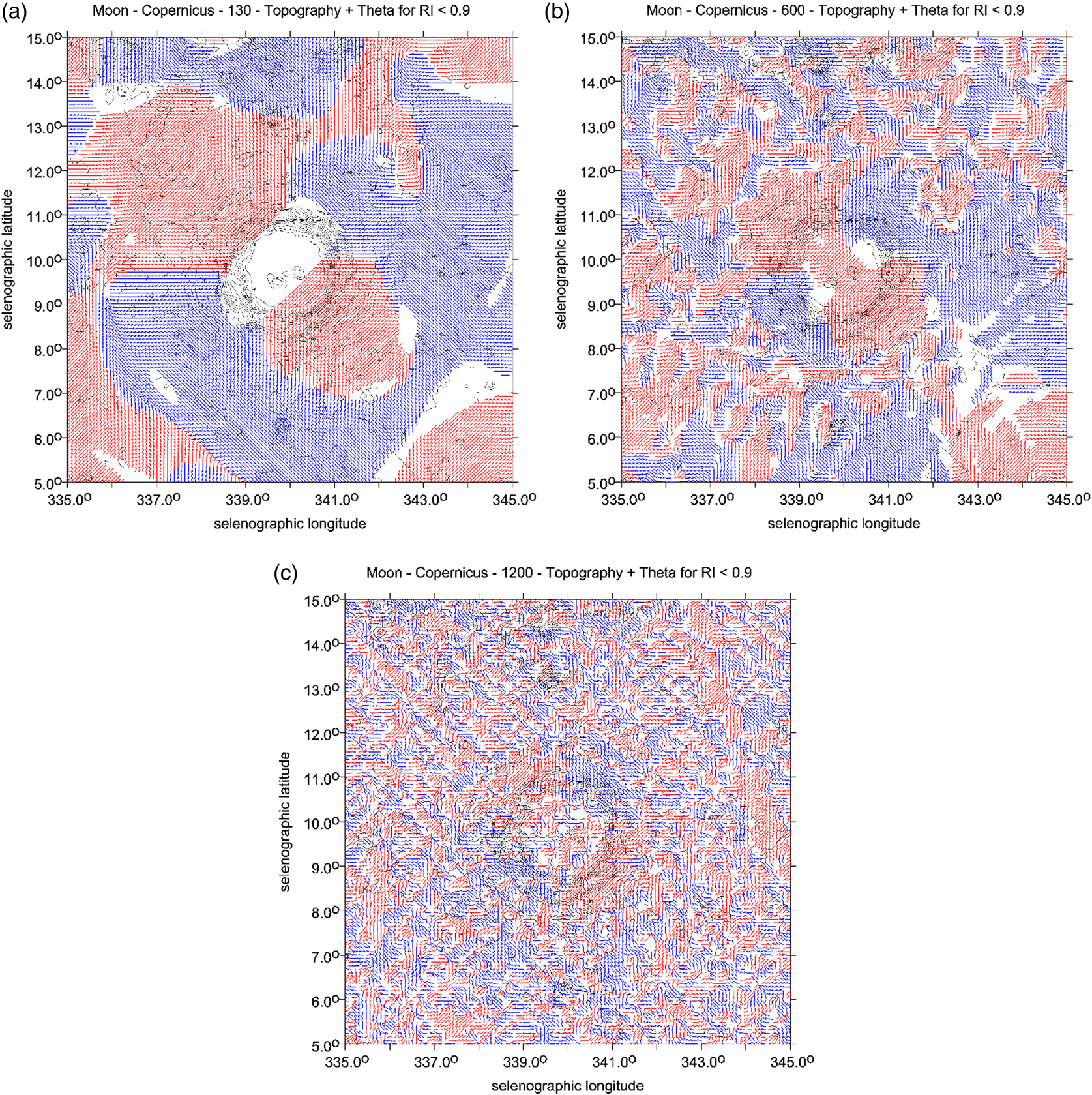
Figure 1. Moon's crater Copernicus, the strike angles, from the gravity model (Konopliv et al., Reference Konopliv, Park Ryan, Rivoldini, Baland, Le Maistre and Van Hoolst2020): (a) cut at d/o = 130 (it is too low, thus losing information); (b) cut at the recommended optimum d/o = 600 and (c) a devastating graining effect appears when d/o is kept up to 1200. Note that the blue and red colours relate to the quadrants of the strike angles. The θ [°] is expressed with respect to the local meridian; the red colour means its direction is to the north and blue is to the south of the east (for more information, see S2: 2).
Figure 1(a)–(c) compare the strike angles computed for I < 0.9 and to d/o = 130, 600 and 1200 for the Moon's crater Copernicus. A loose signal, its resolution, smoothing and generalization for d/o < 600 is evident, and trivial, but what happens for d/o = 1200 may be surprising for the reader (we have many such examples in Klokočník et al., Reference Klokočník, Kostelecký, Bezděk and Kletetschka2021a). The limit d/o = 1200 is too high, the data from the Moon's orbiters are not adequate for such a high limit, and the gravity signal in terms of θ degenerates, and disintegrates due to a (well-known) graining effect into small ‘islands’ (Fig. 1(c)); the halo around the crater then disappears. The consequence is that we only see artefacts, nothing real.
Our conclusions from test 1 for Mars are: (i) to use JGMRO_120F just to d/o = 80, and not higher. (ii) The θ values at the NMPO, being combed into big ‘plates’ (see Section ‘Individual zones/segments in the palaeo-ocean’) are not those small grained ‘islands’ – artefacts, as in Fig. 1(c), but might be the actual features on Mars. Further testing will be useful (tests 2 and 3).
Test 2
The gravity model JGMRO_120F is practically available to d/o = 80 and represents the top-most knowledge now; and it will be much better soon. JGMRO_120F yields the ground resolution of about 130 km on Mars. For the Earth, we also have – in addition to satellite data – terrestrial gravimetric data for effectively high(er) degrees and orders of harmonic coefficients (Stokes parameters) in the combined gravity models. No such analogy exists for Mars; here are ‘only’ the orbits of planetary orbiters and measurements from the on-board laser altimeters.
Let us imagine for a moment that our knowledge about the Earth's gravity field ends at a maximum d/o = 80 (corresponding to the ground resolution of about 260 km in this case). Let us compute and plot θ for this limit and compare the results with the full gravity model (2190). We used gravity EIGEN 6C4 (Förste et al., Reference Förste, Bruinsma, Abrikosov, Lemoine, Schaller, Goetze, Ebbing, Marty, Flechtner, Balmino and Biancale2014), complete to d/o = 2190 (the relevant ground resolution of 9 km). This can be called the ‘true’ gravity field model for this test. There is the question as to what degree the strikes θ will become smoothed, generalized and degenerated with d/o(reduced) and also, whether some of the artefacts, which could be potentially misleading, would arise.
We reply to the questions with Figs. 2(a) and (b) and 3(a) and (b) and S2: 21–39. It becomes obvious that the higher ground resolution means smaller areas of alignment, and that some artefacts appear. Colour dashes (abscissae) show θ for d/o = 2190, and black dashes (abscissae) for 80. While the cut at 80 simplifies the picture too much and omits important features, as must be expected, the general trend of alignment is roughly the same for both d/o = 2190 and 80. This is an encouraging finding, but one has to be very careful to avoid misinterpretations with d/o = 80; there are some artefacts showing a rotation in the alignments for 80 (Fig. S2: 32–34) which the ‘real’, full gravity model, does not confirm.

Figure 2. Cut at a low d/o to simulate a lower resolution of the Martian gravity field models now available, by means of the gravity field EIGEN 6C4, valid for the Earth. The areas are (a) the eastern Mediterranean Sea, and (b) the southern part of the Caspian Sea. Coloured dashes show θ for d/o = 2190, and black dashes (abscissae) for d/o = 80. Our finding based on these tests is: we can rely, with some caution, upon the general trend of alignment because it is roughly maintained from the limit d/o = 2190 down to the cut at d/o = 80. Various disturbing and misleading artefacts are, however, possible, like directional changes of the alignment, false rotation-like features, etc.; see Supplement S2: Fig. S2: 23, 26 or 32–34. Red dots are for deposits of oil/gas (gathered from various sources), incl. L. Eppelbaum, Tel Aviv Univ. (private commun.).

Figure 3. (a) Strike angles for the Earth with the full model EIGEN 6C4 to maximum d/o = 2190. In the window in South America, the alignment of the strike angles is observed in a very limited narrow belt, going along the seashore (~NS direction). This is taken as ‘reality’, as a reference to be now confronted with the cut at a lower d/o in (b). (b) The insufficient knowledge of the gravity field, here modelled for the Earth, simulating EIGEN 6C4 only to maximum d/o = 80. It degrades the strike angles not only due to significantly lower resolution ( = neglecting details) but also due to the origin of unexpected artefacts – in the windows we can see red areas with highly combed strikes while in the ‘real’ field (in Fig. 3(a)) with the d/o to a maximum of 2190, they were reduced or missing. This is a warning example of the treacherous artefacts. (c) The strike angles θ [deg] for the east Mediterranean (EIGEN 6C4 to d/o = 2190), computed for the ratio I = 0.9. A black and white version of Fig. 2(a) without dots giving better view of those large ‘plates’ of aligned areas. Topography relief is derived from the MOLA data. For further figures of this type, see Supplement 2. The strike angles θ [deg] for the Persian Gulf, EIGEN 6C4 (I = 0.9) to (d) d/o = 2190 and (e) d/o = 80. Note the remarkable difference in resolution but a common trend of alignment. The topography relief is from MOLA. Observe closely and mutually compare Figs. 2–4. This test is very important.
Figure 3(a) detects areas on the Earth with the high comb factor – brown contour lines with Comb = 0.95 and also the highest comb factor areas (Comb ≥ 0.99) for d/o = 2190; we can see that they are rare. In Fig. 3(b), we have the same but for d/o = 80, we can see significantly more combed areas here than in Fig. 3(a). Now, we transfer brown contour lines for Comb = 0.95 from Fig. 3(a) into Fig. 3(b). The result is that the red values (for Comb ≥ 0.99), computed from the cut model at d/o = 80, correlate well with the brown contours to d/o = 2190.
The two areas delineated by rectangles in Fig. 3(a) and (b) compare two examples with different behaviour while the comb factor between the solutions to 2190 and 80 is the same. The example of the west border of South America with d/o = 2190 and Comb > 0.95 contains only a narrow belt along the seashore, Fig. 3(a). The result to d/o = 80 (and Comb > 0.95) shows a wider alignment area, reaching far from the seashore, Fig. 3(b). This is false information. There is another situation for the second rectangle in Fig. 3(a), and (b), in Tibet. The model to 80 shows a high alignment there, while the full solution to 2190 does not. This is misleading and can be dangerous for interpretation. In general, however, the trends of the plates with the combed strikes to d/o = 80 reproduce the ‘reality’, i.e. the alignments depicted by the full model 2190, well, ignoring details, over the whole world. We can only hope that the same conclusion will be valid for Mars.
The conclusion from tests 1 and 2 – for sufficiently large ‘plates’ of aligned θ, not affected by graining but also sufficiently extensive to be well above the resolution of JGMRO_120F (i.e. about 130 km ≈ 2.5°) – is that we can rely upon general trends of alignment because they are roughly maintained for d/o = 2190 and d/o = 80 as well. Such ‘plates’ are shown in Fig. 3(c) for the east Mediterranean (to be compared to Fig. 4(c) for Mars) and in S2.

Figure 4. Strike angles θ [deg] for Mars with JPL JGMRO_120F (Konopliv et al., Reference Konopliv, Park Ryan, Rivoldini, Baland, Le Maistre and Van Hoolst2020) to maximum d/o = 80, computed for the ratio I = 0.9. East/west longitude on the x-axis, latitude on the y-axis. (a) The strike angle is expressed with respect to the local meridian; its red colour means its direction to the north and blue is to the south of the east. (b) The Comb statistics – the red colour valid for the highest degree of alignment – Comb ≥ 0.99. (c) Martian dichotomy in the form of a different look of alignments of the gravity strike angles for a part of the Northern and Southern Hemispheres. This is an example of the strike angles in a part of the hypothetical NMPO. We show a contrast between the varied terrain of the highlands on the Southern Hemisphere and the plain, drab ‘sea bottom’ in the lowlands, the Northern Hemisphere. In the lowlands, the strike angles are intensively combed and form large ‘plates’ with one prevailing direction of alignment in the plate. Artefacts cannot be fully ruled out, but our tests (Section ‘Preparatory truncation tests’) show that reality is prevailing. Contours with the MOLA topography are added in the blue colour.
Test 3
To complete the previous tests, we amend Fig. 3(d) and (e); the strike angles θ are shown for the Persian Gulf and Ghawar in Saudi Arabia, using EIGEN 6C4 (I < 0.9) to d/o = 2190 and to d/o = 80. The reader can mutually compare Fig. 3(d) and (e) and these figures to Figs. 2(a), and (b) and 4(c) to see a similarity of large aligned plates of θ for the Earth and Mars for d/o = 80. We derive that the plates in both celestial bodies appear due to the same reason.
We know that the ground resolution of GRGM1200A (a recent gravity field model for the Moon), in use to d/o = 600, is ~10 km. To illustrate the effect of truncation, we cut this model drastically even at d/o = 10, yielding the resolution at only about 600 km. Thus, (i) many details below the limit 600 remain hidden, and (ii) some artefacts are created (see Fig. S2: 39).
The reader can learn more about the danger and character of the artefacts in our specialization from Klokočník et al. (Reference Klokočník, Kostelecký, Bezděk and Kletetschka2021a) and from Fig. S2: 21–38. All of this is mentioned here, because we want to warn against too optimistic interpretations with the present-day gravity field models for any celestial body.
As the conclusion to the truncation tests: even now, with the high-quality and resolution gravity models, we meet artefacts. The history known from the modelling of the Earth's gravity field repeats, but on another, much higher level of quality (a higher resolution). We draw attention to this item because the reader should be aware of it to interpret our results correctly.
Strike angles globally
These are samples of our global views on Mars with the gravity model JPL JGMRO_120F (Konopliv et al., Reference Konopliv, Park Ryan, Rivoldini, Baland, Le Maistre and Van Hoolst2020) to a maximum d/o = 80 showing the strike angles without (Fig. 4(a)) and with the comb statistics – the red areas in Fig. 4(b) have Comb > 0.99. For gravity aspects other than the strike angles, see Supplement 3 (Fig. S3: 4–9).
It looks like (Fig. 4(a) and (c)) the large areas (looking like ‘plates’) in the northern lowlands are highly combed. Figure 4(b) shows clearly that the highest alignment exists more frequently over the lowlands (mostly plain, drab terrain) than on the highlands (with more varied terrain). The strike angles thus confirm a conspicuous difference between the northern and southern parts of the globe of Mars and not only in the topography (well known). While Δg, Tzz and the invariants support the fact of a gravitationally, relatively ‘silent’ area (dumped due to the effect of thick sediments?) for the northern part, but not everywhere, θ and vd disclose more: a difference in porosity (higher in the lowlands) and various stress tendencies (higher in the highlands).
Strike angles for the polar areas
The northern cap (MOLA topography relief in Fig. 5(a)) is bigger and mostly comprised of ice water (H2O), while the southern is mostly CO2 (Fig. 6(a)), but water is present there, too (e.g. Arnold et al., Reference Arnold, Butcher, Conway, Gallagher and Balme2022). Both have a higher porosity than the surrounding rocks. This should be reflected in the strike angles that would be aligned.
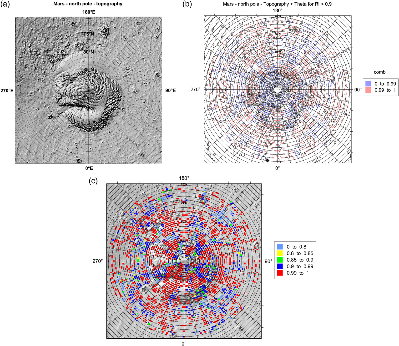
Figure 5. (a) MOLA topography relief (m) for the northern polar cap. ‘Dunes’ and ‘rotation’ due to Coriolis force are well visible. More about the interpretation to the series of Figs. 5 and 6 is provided in Discussion. (b) The strike angles (I < 0.9) in the form of Comb factors, in a combination with abscissae for the strikes. MOLA contour lines are added. (c) The strike angles (I < 0.9) in the form of Comb factors. Together with the MOLA height profile.

Figure 6. (a) MOLA topography relief for the southern polar cap. This cap is smaller than the northern cap, but the extent of latitudes on this scale differs from that in Fig. 5(a); in turn this cap may look more massive. (b) The strike angles (I < 0.9) in the form of Comb factors, in a combination with abscissae for the strikes. MOLA contour lines added. (c) The strike angles (I < 0.9) in the form of Comb factors. Together with the MOLA height profile.
Here, we show the topography and strike angles only. The other gravity aspects are provided in Supplement 3, see Fig. S3: 69–81. Figures 5(b) and (c) and 6(b) and (c) show the relevant strike angles for the northern and southern caps. The reader can see that the alignment is (i) conspicuous for both caps, that (ii) the alignment is not so extreme on the south (cf. Fig. 6(c) to Fig. 5(c), note that the colour scales of these figures are the same) and (iii) the northern cap is more aligned than the surrounding NMPO.
Figure 5(a), showing the surface morphology, has two basic features – smooth and rugged surfaces. Both can be interpreted as manifestations of wind activity. The strike angles in Fig. 5(b) complement this information. Figure 5(b) shows beneath the planet's surface. The relatively low density of the gravimetric signal means that the diagram captures the basic most prominent features of the mass structure of the polar region of Mars. Terrestrial analogies, verified, e.g. by drilling and geophysical work and measurements, have repeatedly shown that gravimetry is capable of capturing the geological structure at a range of at least 2–5 km below the surface.
The spiral structure corresponding to the morphology is quite visible in a rough outline in Fig. 5(b). This probably indicates that similar aeolian processes have been operating on Mars for a long time. The whole scheme can be decomposed into approximately concentric features, which probably correspond to aeolian processes caused by planetary rotation (Coriolis force), and radial structures, which are not visible in the morphology in Fig. 5(a). The seven most pronounced structures lie between 200 and 210°E, but less pronounced lines can also be found at other locations, e.g. between 110 and 120° (see Fig. 5(c) as well). Our explanation is that here we have buried valleys formed by melt water erosion.
The southern polar region already confirms the hypothesis of radial erosion valleys on the geomorphological map (Fig. 6(a)). Note, however, that the position of the strike angles (Fig. 6(b) and (c)), e.g. between 60 and 70°E or between 300 and 320°E, does not correspond to the present morphology of Mars. This may indicate that another, older and somewhat different set of erosional features lies beneath the present valley network.
We consider the test for the polar caps of Mars as a very useful ‘test-bed’. We receive what we expected. This means that we have checked that (i) the strike angles are highly combed (due to the higher porosity of material of the caps). Moreover, we verified that (ii) the northern, bigger and thicker cap is more intensively combed than the southern.
Similar situations with highly combed areas but not uniquely focused on the causative bodies, are known from the Earth (Section ‘Introduction’) for groundwater, subglacial features, canyons, palaeo-lakes, oil and gas deposit localities and also, in a circular form (as a halo), for impact craters and basins (and this is also true for the Moon, see Klokočník et al., Reference Klokočník, Kostelecký, Cílek, Kletetschka and Bezděk2022a).
Thus, we conclude that the concept of the strike angles ‘works well’, and that it ‘works as should work’, so we can do the next step of our analyses.
Extent of the palaeo-ocean
Discussion about a hypothetical ocean or oceans (Arabia, Deuteronilus, Oceanus Borealis or Utopia, its part) on Mars is old (e.g. Baker et al., Reference Baker, Strom, Gulick, Kargel and Komatsu1991; Parker et al., Reference Parker, Gorsline, Saunders, Pieri and Schneeberger1993; Head et al., Reference Head, Hiesinger, Ivanov, Kreslavsky, Pratt and Thomson1999; Clifford and Parker Reference Clifford and Parker2001; Ghatan and Zimbelman Reference Ghatan and Zimbelman2006; Forget et al., Reference Forget, Costard and Lognonné2008). The ocean would cover the vast topographically low plains of Vastitas Borealis, Chryse, Arcadia, Acidalia and Utopia Planitia. The topography and the gravity aspects do not in general correlate as we would expect for the Earth at least for the gravity anomalies; these low areas are not ‘silent’ everywhere in terms of the gravity signal (see series of Figs. 4 and S3: 4–9, 21–66).
Since the early discovery of Martian north-south topographic dissymmetry or dichotomy, it has been logical to put a putative palaeo-ocean or oceans, lakes and rivers mostly towards the topographically low northern plains, like the Vastitas Borealis formation – looking like abyssal plains of the Earth's oceans (e.g. Carr and Head, Reference Carr and Head2003; Irwin and Watters, Reference Irwin and Watters2010). The rugged frontier, the transition zone in between the lowlands and highlands, known as fretted terrain, may define a part of the seashore (Forget et al., Reference Forget, Costard and Lognonné2008). But the shore is highly topographically variable, so we have to refer to one equipotential level (Lemoine et al., Reference Lemoine, Smith, Rowlands, Zuber, Neumann, Chinn and Pavlis2001; Smith et al., Reference Smith, Zuber, Frey, Garvin, Head, Muhleman, Pettengill, Phillips, Solomon, Zwally, Banerdt, Duxbury, Golombek, Lemoine, Neumann, Rowlands, Aharonson, Ford, Ivanov, Johnson, McGovern, Abshire, Afzal and Sun2001; Zuber, Reference Zuber2018). It is important to recall that the MOLA MGS topography is related to the global Mars' best-fitting ellipsoid and, in turn, to the particular gravity field model and Mars' geoid-areoid, in other words, to an equipotential surface (Section ‘Gravity and topography data and reference ellipsoid’).
In this experiment, we ignore any knowledge in the first step about the geological features and history of Mars and all previous attempts to delineate the extent of the palaeo-ocean. Constraints on estimating its hypothetical seashore are derived with the aid of the global MOLA topography (Fig. 7(a)–(e)), going from the southern highlands, using knowledge of geographical locations of the fretted terrain via the northern lowlands to the northern polar cap. The real seashore was evidently time variable (due to various reasons) during the long history of Mars – before the NMPO had desiccated after all. A more fragmented potential shoreline can be expected.

Figure 7. (a) Global view on Mars with the MOLA topography (in (m)). The estimated ‘seashore’ of the NMPO is expected to be between −3000 and −4000 m. The red contour line corresponds to −3500 m. The border between the Northern and Southern Hemispheres contains in various places the fretted terrain, described in the literature. For us, it is important that the erosion that formed the fretted terrain was aided by water (e.g. Denton and Head, Reference Denton and Head2018). For comparison see, e.g. Kite et al. (Reference Kite, Rafkin, Michaels, Dietrich and Manga2011). (b) The northern polar cap on Mars by means of the MOLA topography (m). The tentative ‘seashores’ of the NMPO at various levels. (c) MOLA topography (m) for the Valles Marineris (VM). A possible connection to the hypothetical palaeo-ocean – its seashore is shown by the red contour line (for −3500 m). The numbers in the yellow colour localize black dots in (d). (d) The altitude profile of the VM from the west (Tharsis) to the east and north (NMPO), points 1–13 in (c). The distance on the x-axis is computed from point 1. Based on MOLA topography (m). (e) A compromise for the ‘seashore’ line found: the height may be ~−3500 m with respect to the reference ellipsoid, this is our model altitude for the hypothetical seashore of the hypothetical palaeo-ocean. Based on the MOLA topography (m).
Figure 7(a) yields −3000 to −3500 m for such a model seashore altitude, while the topography at the cap in Fig. 7(b) leads rather to −4000 m.
In the second step, we account for previous attempts to delineate the palaeo-ocean and for the generally accepted geological history of Mars (e.g. Irwin and Watters, Reference Irwin and Watters2010; Citron et al., Reference Citron, Manga and Hemingway2018a, Reference Citron, Manga and Tan2018b). The palaeo-ocean belongs to the Noachian era (from the planet's formation to 3.5 billion years ago, Gy), after some time desiccating. The cap should be newer – late Amazonian (~1 Gy). The fretted terrain is Noachian-Hesperian. We should not combine the polar cap and the lowland–highland border as a common condition for the height of the seashore. We should prefer to use the older features (Fig. 7(b)). Then, we cannot be surprised that, for example, at the height of −3000 m, the northern polar cap would be partly ‘flooded’ (Fig. 7(b)).
To compare our results, we used the estimate from Forget et al. (Reference Forget, Costard and Lognonné2008), based on the MOLA data, too. Their estimate is the seashore at −4350 m ‘above the zero level’ (which we hope is the same ellipsoid as in our case, Section ‘Gravity and topography data and reference ellipsoid’). The ocean might be 600 m deep.
As a check, Fig. 7(c) (a connection between the NMPO and the Valles (valleys) Marineris (VM) on a level at −3500 m) confirms that this choice is appropriate; compare Fig. 7(c) to (a), see Fig. S3: 11–19.
Figure 7(d) is an altitude profile of the VM from west to east and then to the north (follow points 1–13 in Fig. 7(c)). We can see (i) a general trend of topography from the top-down from west to east and to the flat ‘delta’ north, and (ii) we can speculate about a deeper lake in the VM between points 3 and 6 and hypothetical rapids or waterfalls or both between 2 and 3 or 9 and 10. There are terrestrial analogies where long valleys break up into sub-basins, in some periods. The headlands between the basins are either of tectonic origin or have been formed by filling with sediments from lateral tributaries or landslides.
After all the experimenting, our final estimate for the seashore height (giving its hypothetical long-term level) is about −3500 m.
Individual zones/segments in the palaeo-ocean
Six segments over the hypothetical NMPO are shown here, from west to east, based on the MOLA topography and the gravity strike angles from JPL JGMRO_120F (Konopliv et al., Reference Konopliv, Park Ryan, Rivoldini, Baland, Le Maistre and Van Hoolst2020), see Section ‘Gravity and topography data and reference ellipsoid’, to d/o = 80. The other gravity aspects (Δg, Tzz, Ij, I, θ and vd, and the MOLA topography) can be found in Supplement S3 as Fig. S3: 20–67.
For a better orientation on Mars, we recommend using the USGS (2003) topographic map of Mars. For a few comments on the strike angles of the individual segments, see in Section ‘Strike angles’ map documentation’.
This series of figures with the strike angles for the individual zones mostly for the northern lowlands clearly demonstrates highly aligned strikes. We will quantify the degree of their alignment by means of the comb factor and tentatively interpret these results in Section ‘Strike angles’ map documentation’.
Criteria
In an analogy to the Earth, we seek the largest and highest combed areas of θ giving a higher chance for hydrocarbon reservoirs. We suggest that promising oil areas could be located at an intersection of three basic factors:
(i) The ocean, as a larger body of water, which has a fairly significant thermal and chemical inertia. It is, therefore, not subjected to rapid changes that could threaten emerging life.
(ii) The existence of a thermal oasis containing substances that are capable of providing energy. These places are suitable for the evolution of chemotrophic bacteria. They can be detected as chemofossils containing a wide range of substances such as: hydrocarbons, iron oxides, sulphates, carbonates, etc. On the Earth, these sites are typically associated with fault structures related to mid-ocean ridges and other areas of increased volcanic activity.
(iii) A suitable place where chemofossils indicated by hydrocarbons could be preserved (oil traps).
We prefer areas in the NMPO, which are as large as possible, together with combed strike angles that are as high as possible. But such an inland sea like the Hellas basin probably also poses ground (ice) water. Within our first estimate, we focus on the NMPO. We know from Sections ‘Gravity and topography data and reference ellipsoid’ and ‘Preparatory truncation tests’ that the ground resolution, dictated by the gravity model JGMRO_120F (not by the method), is about 2.5°. Thus, we will ignore all (even very well combed) areas smaller than 10°, at least in one dimension (harder than the criterion ~3σ). Further, we select only the red zones of θ with Comb ≥ 0.99.
We know that for oil fields, but also for the areas where groundwater reservoirs exist, a combed structure with a parallel course of strike angles is typical. These structures on the Earth indicate places where underground reservoirs or oil traps are not disturbed by newer folding or fault tectonics. Thus, we prefer ‘gravitationally silent’ areas, meaning areas without sharp changes in Δg, Tzz or the invariants. This prefers flatter sedimentary areas, but proximity to volcanoes or trenches can also not be excluded, if Comb ≥ 0.99. The sediments, superimposed upon the pre-existing surface features, reduce Δg, Tzz (much more for Tzz and the invariants than for Δg) of those underlying structures, and affect the orientation of θ and vd.
The zones fulfilling our criteria are selected and presented with a commentary in the next section. The reader can perform her/his own selection according to her/his criteria from our results in Sections ‘Strike angles globally’, ‘Strike angles for the polar areas’ and ‘Individual zones/segments in the palaeo-ocean’.
Strike angles' map documentation
The results from Section ‘Individual zones/segments in the palaeo-ocean’ are now presented in the form of colour maps of the strike angles in Fig. 9(a)–(f) with the Comb factors (explained in Section ‘Method’), and in another projection. The selected features in Fig. 9(a)–(f) are discussed. The ovals indicate the largest areas with the highest Comb value (in red colour) in the respective segment. Names are according to the Topographic Map of Mars (USGS, 2003).
Particularly striking are the elongated anomalies, which usually have a red centre and a narrow blue rim. They are found especially at 50°N and −130°, 50° and −100° or in the southern part of the figure at 30°N and −150° to −120°. The continuation of the valley, oriented NE, at 50°N and −60°, which clearly represents the outflow area, opens up an interpretative possibility. Similarly, the elongated anomalies can be considered as the remains of broad streams or flow-through lakes.
The most striking feature of Fig. 9(b) is the large homogeneously arranged area around the VM. The analogous valley structure in the upper right corner (Sydonia Mensae) can also be used for its interpretation. We assume that it could be a fairly uniformly deposited sediment on tilted blocks of rift or tectonic blocks. Aeolian-transported or washed sediments can cause softening of the originally much more rugged relief. However, this depends on the prevailing wind direction, i.e. on the local climate, where the thicker sedimentary layers will form.
In the VM, one can surprisingly see the highest Comb values in the fault and in its wide surroundings along the fault, perhaps a real feature, not an artefact (Fig. 9(c)). One possible explanation is that there was a uniform deposition of aeolian and slope sediments on the long, inclined surfaces around the central rift. In the same figure, notice the ends of shallow valleys that merge into the sea basin (10°S–15°N, 50–20°W). This is a typical area where, in our opinion, we can look for occurrences of hydrocarbons.
From an interpretative point of view, it is appropriate to move from Figs. 9(c) to 3(c), which shows the Nile delta. The Nile Valley itself has an orientation of strike angles in the direction of the structure, but the delta grew gradually and was modelled by sea currents, so its orientation is perpendicular to the direction of the river. The direction of the combed θ follows the course of the long axis of the VM, as the reader expects.
It is not easy to interpret Fig. 9(c)–(f) either, but the most important features of the relief are neither striking craters like on the Moon nor linear structures like on the Earth; instead, we encounter more or less regular surfaces. Thus, there is no evidence of a clear river network manifested by well-defined valleys. Instead, broad, elongated anomalies appear in places. It is thought that this type of structure was mainly formed by aeolian processes, but on the whole the fine-grained sediments were periodically moved during wetter or more humid periods. This situation can be approximately compared to the present-day shallow Lake Chad Basin or to some Triassic formations of the US Midwest.
Summary of our observations and discussion
The strike angles in the northern lowlands of Mars are combed nearly everywhere and often more intensively than on the Southern Hemisphere (Figs. 4(a)–(c), 5(c) and 8(a), (b) and (d); S3: 7, 8, 73–75, 79–81). The strong alignment relates mainly to the NMPO. It corresponds to a higher porosity of the material, meaning the sedimentary layer, ground-ice (permafrost), groundwater sources, oil-type/hydrocarbon occurrences, lahars, palaeo-lakes, deltas of hypothetical rivers (e.g. Fig. 7(c)), fretted terrain (Figs. 8(c) and (d) and 9(c), (d) and (f)) or the relative vicinity to volcanoes and lahars (Fig. 8(a) and (f)).

Figure 8. (a) Topography (MOLA (m)) and the strike angles θ (for I < 0.9) for the selected zone. The feature at (φ = 40°N, λ = 110°W) is Alba Patera near Olympus Mons. 1° ~ 50 km. (b) Topography (MOLA (m)) and the strike angles θ (for I < 0.9) for the selected zone, mainly the Valles Marineris (VM). The feature at (7°N, 22°W) is the crater Aram Chaos. A halo-like shape of several features north of the VM resembles smaller volcanoes. (c) Topography (MOLA (m)) and the strike angles θ (for I < 0.9) for the selected zone, partly Arabia Terra (bottom right). The feature at (65°N, 10°W) is the crater Lomonosov in the Vastitas Borealis plain. Here, the reader can compare colour and black and white versions of the figure for the same zone. (d) Topography (MOLA (m)) and the strike angles θ (for I < 0.9) for the selected zone. The feature at (50°N, 30°E) is the crater Lyot, north of the Deuteronilus Mensae fretted terrain. (e) Topography (MOLA (m)) and the strike angles θ (for I < 0.9) for the selected zone. The feature, bottom left is Isidis Planitia, with an approximately hexagonal shape, the plains EN of it are a part of Utopia Planitia. The landing site of Perseverance is shown by the white star. (f) Topography (MOLA (m)) and the strike angles θ (for I < 0.9) for the selected zone. The feature at (25°N, 145°E) is Elysium Mons.

Figure 9. (a) Feature at (φ = 40°N, λ = 110°W) is Alba Patera near Olympus Mons (on the southern edge of this figure). The oval with the largest area with the highest Comb is located near a crater (with the misleading name of Erebus Montes) partly buried in sediments in Amazonis Planitia, NW of Olympus; see also the slides with other gravity aspects – Fig. S3: 20–31 in Supplement 3. The slant ‘rifts’ at (φ = 25–45°N, λ = 90–60°W) belong to Mareotis Fossae and Tempe Fossae. (b) The highest Comb values along the Valles Marineris (VM) and within its wide surroundings. This might, however, be an artefact like those shown in Section ‘Preparatory truncation tests’; compare (b) to Figs. 3(a) and (b); we cannot exclude this possibility. Tharsis would be on the left-hand side (outside). The crater at [φ = 7°N, λ = 22°W] in the ‘delta’ of the VM to the hypothetical NMPO (via Chryse Planitia) is Aram Chaos. The red belt at the upper right-hand corner belongs to Sydonia Mensae. (c) The ovals are (top-down) in: (1) Vastitas Borealis lowland [φ = 65–75°N, λ = 40–0°W]; the crater Lomonosov at (65°N, 10°W); (2) the lowland part at Acidalia Planitia [φ = 35–50°N, λ = 30–5°W]; (3) on the border between lowland and highland, Cydonia Mensae [φ = 25–45°N, λ = 20–0°W]. (d) The oval at [φ = 50–60°N, λ = 35–60°E] is in the lowlands, crater Lyot is at [φ = 50°N, λ = 30°E], Deuteronilus Mensae is at [φ ~ 40°N, λ = 10–60°E] and Arabia Terra is south of this. (e) Utopia Planitia [φ = 50–60°N, λ = 85–120°E]. Isidis Planitia [φ = 0–20°N, λ = 75–100°E]. (f) Elysium [φ = 20–30°N, λ = 125–140°E]; see also Fig. S3: 67. Gale crater at [φ = 5°S, λ = 138°E]; Apollinaris Pater volcano at [φ = 9°S, λ = 175°E].
The combed strike angles θ in the NMPO create features like ‘plates’ on the surface (large areas, zones and belts that can be 20° across) keeping a similar orientation of θ in the given plate (a series of Figs. 8(a)–(f); S3: 28, 29, 37–39, 46, 47, 55–57, 64, 65, 75, 81, 84). It appears that the plates do not in general correlate with the other gravity aspects, e.g. a high porosity does not automatically mean a low density, because it may be masked by various geological features beneath the sedimentary layer. The strikes react dominantly on the sediment and not on deeper layers.
We confirm that the polar caps are highly combed, the northern more than the southern (Fig. 5(b) and (c) versus 6(b) and (c), S3: 73–75, 79–81). The northern cap exhibits more intensive alignments than the NMPO as a whole.
The Isidis basin (Figs. 8(e), 9(e) and S3: 49–59, 86–88) would be a part of the edge of the NMPO. Around the Isidis basin, magnesium carbonate was discovered (by the MRO); this indicates non-acid water with favourable conditions for the evolution of life (Murchie et al., Reference Murchie, Mustard, Ehlmann, Milliken, Bishop, McKeown, Noe Dobrea, Seelos, Buczkowski, Wiseman, Arvidson, Wray, Swayze, Clark, Des Marais, McEwen and Bibring2009). Nearby, in Utopia Planitia, a part of the NMPO, groundwater was detected (by radar on the MRO, Section ‘Introduction’). The Zhurong rover of China's Tianwen-1 mission, which landed in southern Utopia Planitia, identified hydrated sulphate/silica materials on the Amazonian terrain at the landing site (Liu et al., Reference Liu, Wu, Zhao, Pan, Wang, Liu, Zhao, Zhou, Zhang, Wu, Wan and Zou2022). The locality fits well with the place with the highest Comb factor in Fig. 9(e). We should remember that when comparing such results with ours one has to be aware of the ground resolution accessible by us (dictated by the gravity field model used) and that it is about 130 km.
At the west-north of Tharsis (at φ = 35°N, λ = 170°S), there is a big crater nearly entirely buried under sediments, but well visible in the gravity aspects (Fig. 8(a) with θ but better in Fig. S3: 20–31).
In the Valles Marineris (VM), one can surprisingly see the highest Comb values in the fault and in the wide surroundings along the fault, perhaps a real feature, not an artefact (Fig. 9(c) and S3: 100–103). One possible explanation is that there was a uniform deposition of aeolian and slope sediments on the long, inclined surfaces around the central rift. In the same figure, notice the ends of shallow valleys that merge into the sea basin (10°S–15°N, 50–20°W). This is a typical area where, in our opinion, we can look for occurrences of hydrocarbons.
We investigated a possible extent of the NMPO (Section ‘Extent of the palaeo-ocean’). We used MOLA topography for a hypothetical seashore, the northern polar cap and the VM as a hypothetical river flowing to the VM from Tharsis Plato (series of Fig. 7). Figure 7(d) shows an altitude profile of the VM from west to east and north (with a hypothetical delta or deltas), confirming a general trend of topography from the top-down for running water, leaving space for speculations about deeper lakes, rapids or waterfalls along the trench. Here we recall Fig. 7(c) for the height profiles to the height profiles in Section ‘Extent of the palaeo-ocean’. Among many other places, the VM contains sulphates on its floor and walls (according to the Mars Express orbiter camera, combining a spectroscope and imaging device); sulphates require liquid water in their formation (Viviano-Beck et al., Reference Viviano-Beck, Seelos, Murchie, Kahn, Seelos, Taylor, Taylor, Ehlmann, Wisemann, Mustard and Morgan2014).
Potential hydrocarbons are more likely to be found in places with ordered combed structures, which probably represent here places with linear (uniform) water flow, as on Earth that would carry and concentrate hydrocarbon chemofossils in suitable places, e.g. under impermeable clay layers.
In interpreting areas with aligned strike angles, we so far mainly considered the overflow of fine-grained aeolian material, but there are other possibilities. These include dry granular flows, which are known on Earth and could be even more abundant on Mars given the height of the volcanoes and a lower gravity. Such terrain might be dangerous for future astronauts.
It turns out that the gravity aspects are sensitive not only to uniformly ordered sediments of shallow basins (the ‘plates’), but also to the supposed lahars (‘mud flows’), provided that the area covered by them is above the ground resolution limit of the gravity field model (in our case ~130 km). They were described on Mars more than 40 years ago and are further studied (Allen, Reference Allen1979; Christiansen, Reference Christiansen1989; Cuřín et al., Reference Cuřín, Brož, Hauber and Markonis2023) recently amended by laboratory experiments (Brož et al., Reference Brož, Krýza, Wilson, SJ, Hauber, Mazzini, Raack, MR, ME and MR2020).
Pedersen (2013 and a set of references in this paper) writes that ‘intrusions have been proposed as mechanisms for generating major lahars in various regions…’ [roughly for orientation at: φ…°N or S, λ…°E], such as Mangela Valles [10S, 210], Elysium Fessae/Fossae [25N, 140], Cerberus Fessae [10N, 165] and Athabasca Valles [10N, 155], ‘…either by melting a substantial amount of ground ice or by cracking the cryosphere allowing drainage of confined aquifers…’ and ‘…a plethora of volcano–ice interactions known from Earth have been suggested to occur on Mars, and the transition zone between the Elysium rise and Utopia Planitia has been commonly suggested to host a variety of these features…’; he studied these morphologically complicated features in detail (Pedersen, Reference Pedersen2013).
We have checked, using our figures in the main text and in S3, together with topography maps, that for example the huge Elysium lahar field [~30, ~135], situated approximately west of the Elysium volcano (Fig. 9(f); S3: 50–59), belongs to the areas with the highest Comb factor. These plates are large enough (~1000 km) to be well above our ground resolution (~100 km).
Conclusions
Two sources of remote-sensing data (the gravity aspects, derived from the gravity field models of Mars) (here JGMRO_120F to the d/o = 600), computed from orbits of the Mars orbiters (artificial satellites of Mars), and the surface topography of Mars (MGS MOLA), are used to identify and discuss various geological features on Mars (Section ‘Gravity and topography data and reference ellipsoid’). The gravity aspects enrich views attainable singly by means of the traditional gravity anomalies Δg. The gravity aspects can disclose much more than Δg would manage alone.
(1) ‘We are working here (and have been working during the last decade for the Earth) with functions of the disturbing gravitational potential called gravity aspects (descriptors), broadening the gravity anomalies. The gravity aspects are sensitive in various ways to the ground lithological density contrasts (variations) and stress field orientation due to the causative bodies. These functions, altogether, provide much more complete and thorough information about the causative bodies than the traditional gravity anomalies…’ (quoting from Klokočník et al., Reference Klokočník, Kostelecký, Cílek, Bezděk and Kletetschka2022d). Success also depends on the density contrast in question and (of course) on the ground resolution.
We use the following gravity aspects: the gravity anomaly (or disturbance) Δg, the Marussi tensor (Γ) of the second derivatives of the disturbing potential (Tij), with two gravity invariants (Ij), their specific ratio (I), the strike angles (θ) and the virtual deformations (vd). They are all derived from the global gravity field models for the body (here Mars); they are expressed in terms of harmonic geopotential coefficients (Stokes parameters) to some maximum degree and order (d/o) in their spherical expansion. The ground resolution of the model JPL NASA JGMRO_120F for Mars is about 130 km. This dictates the resolution of the whole method as applied for Mars in the present time (Sections ‘Gravity and topography data and reference ellipsoid’ and ‘Method’). The MOLA topography data in our use have the resolution 0.25° (Section ‘Gravity and topography data and reference ellipsoid’).
Reservoir source rocks are porous, absorbent and can be saturated with water, oil and gas in various combinations. There is an adequate gravity signal; especially for θ this means it has significant and extensive alignments (combed strike angles). We investigated strike angles for oil-bearing regions on the Earth (Klokočník et al., Reference Klokočník, Kostelecký, Bezděk and Kletetschka2021a). We found that oil/gas or groundwater reservoirs are more often located in the areas of large strike angle alignments, where porous masses helped to form oil traps but the seals of these oil traps at depth were not significantly disturbed by brittle tectonics. Mars may contain subsurface deposits of oil and natural gas indicating its past life if it possessed an Earth-like biosphere in the past. We contribute to the discussion in a very unusual way – with the global gravity data watching for the gravity signal (in the form of the gravity aspects) generated by the density contrast, using especially the strike angles. Rivers, canyons, faults, groundwater or ice, permafrost (regolith), palaeo-lakes, oil and gas deposits (more generally hydrocarbons), sedimentary layers, mud – their appearance is signalled by the combed (aligned) strike angles θ, one of the gravity aspects (Section ‘Method’), and of course, in a specific way, by the other gravity aspects. This is not only a reaction to a higher porosity of that place in comparison with its surrounding, but also a reaction to a certain flow, tension, a force connected with such a genesis and evolution of such features. For a 2D-like body rather than for a 3D-like causative (underground) body (density contrast), the combed θ (with a small ratio I, usually below 0.3) means the main direction of the Marussi tensor.
(2) We performed tests (Section ‘Preparatory truncation tests’) to increase confidence that we were studying the real features on Mars and not artefacts. We confirm that (i) we have to use the gravity model JGMRO_120F just to a maximum d/o = 80, not to a higher d/o due to a danger of artefacts known as graining. The truncation tests for the Earth's features and the strike angles with the gravity model EIGEN 6C4 up to d/o = 2190 and only to d/o = 80 show (ii) conspicuous differences: there are sometimes potentially misleading and dangerous artefacts (with d/o = 80 in contrast to 2190). This indicates that future gravity models for Mars with better resolution might reveal (besides losing some details) a completely diverse picture of the distribution, shape and intensity of the combed strike angles. Thus, our present-day interpretations can be biased. However, a general trend of the alignments in those large scales is the same or similar for both cuts – at d/o = 2160 as well as at d/o = 80 (Fig. 2(a) and (b); S2: 21–31). This is an optimistic conclusion, but interpretation must be careful and alert.
(3) The strike angles confirm a conspicuous difference between the northern and southern parts of Mars (Section ‘Strike angles globally’) which is very well known from other studies. The very large plates of the strike angles in the northern lowlands are highly combed, more than in the highlands on the Southern Hemisphere (Fig. 2(a) and (b); S2: 21–31). A still higher alignment is observed for the northern polar cap (Section ‘Strike angles for the polar areas’). While Δg, Tzz and the invariants support the fact of gravitationally, relatively ‘silent’ areas in the lowlands (partly dumped due to the effect of thick sediments), but not everywhere, θ and vd disclose much more: a difference in porosity (higher in the lowlands) and various stress tendencies (higher in the highlands). This can be a sign of ground (ice) water or hydrocarbons or both.
(4) Our estimate of the possible maximum extent of the palaeo-ocean (NMPO) is constrained mainly by the MOLA topography (series of Fig. 7, Section ‘Extent of the palaeo-ocean’; Fig. S3: 11–13, 89–96) and recognizing the difference in the strike angles between the Northern and Southern Hemispheres (e.g. Fig. 4(c)). We found the seashore altitude at −3500 m (above the reference surface, defined in Lemoine et al., Reference Lemoine, Smith, Rowlands, Zuber, Neumann, Chinn and Pavlis2001; Smith et al., Reference Smith, Zuber, Frey, Garvin, Head, Muhleman, Pettengill, Phillips, Solomon, Zwally, Banerdt, Duxbury, Golombek, Lemoine, Neumann, Rowlands, Aharonson, Ford, Ivanov, Johnson, McGovern, Abshire, Afzal and Sun2001) to be valid for some, unknown time interval, but the complicated border was changing due to more reasons (not investigated here).
(5) Then we focused on the palaeo-ocean (NMPO) and divided it into six zones (segments) to see more details in θ. We suggested criteria for the selection of candidates of oil-type or oil/water or hydrocarbon deposit sites (Section ‘Criteria’) and applied them (Section ‘Strike angles’ map documentation’). For extremely combed θ, where a combination of oil and water is predicted, the areas are looking like huge plates and have the factor Comb approaching 1 (in red colour).
(6) Our procedure (the use of the gravity aspects), based dominantly on aligned (combed) strike angles, is not able to pinpoint locations of possible hydrocarbons on Mars, but could serve as a refinement criterion for further geo-research and as additional pre-drilling information telling us about a higher probability of the presence of oil/gas/water/mud/hydrocarbon occurrences in the area. What can be found may not be locations of the deposits, but sites with a chemical signal of the past life on Mars, alternatively the best places on Mars to look for possible traces of past life.
Probably the most important, albeit hypothetical, geological finding is the observation that at least one older relief, formed by similar processes, lies beneath the present Martian surface under study, which has been largely shaped by exogenous aeolian and hydrological processes. This did not form a clearly defined river network with deep valleys, but rather flat flow basins probably formed mainly by sheet flow.
The most promising areas for hydrocarbons on Mars are shown by ovals in Fig. 9(a)–(f). In the Valles Marineris, one can see that the highest Comb values inside and around (10°S–15°N, 50–20°W), also yielded a candidate for occurrences of hydrocarbons. The lahars at volcanoes, like Elysium, belong to the candidates, too.
(7) This additional remote-sensing tool is a cheap one. No additional, special equipment or investment is required – it is ‘just’ necessary to know the generic gravity field model (based on previous measurements of Mars orbiters by others) and to have the relevant software able to compute all of the necessary functions (and to do it safely with numerical stability to high degrees and orders). We have developed such software during the last 10 years or so and have tested it on the Earth and the Moon. The data, computations and figures – for any area of interest – can be provided on request.
(8) The existence of a palaeo-ocean and possible hydrocarbons on Mars provides indication of the past life. The understanding of the situation of water, palaeo-ocean(s) and hydrocarbons on Mars is vital for understanding the evolution of Mars and for its future human exploration (e.g. Robert and Bushnell, Reference Robert and Bushnell2016). The next decade of exploration on Mars prioritizes research into the chemistry, distribution and origin of organic matter in geologic materials. The discovery of biological building blocks in Martian organic matter, present or past, could revolutionize our understanding of the origin of life.
Supplementary material
The supplementary material for this article can be found at https://www.asu.cas.cz/~jklokocn/Hydrocarbons-on-Mars_2023_supplements/.
Data
The gravity field parameters of JGMRO_120F and the MOLA topography are generic (Lemoine et al., Reference Lemoine, Smith, Rowlands, Zuber, Neumann, Chinn and Pavlis2001; Smith et al., Reference Smith, Zuber, Frey, Garvin, Head, Muhleman, Pettengill, Phillips, Solomon, Zwally, Banerdt, Duxbury, Golombek, Lemoine, Neumann, Rowlands, Aharonson, Ford, Ivanov, Johnson, McGovern, Abshire, Afzal and Sun2001; Konopliv et al., Reference Konopliv, Park Ryan, Rivoldini, Baland, Le Maistre and Van Hoolst2020). Our gravity aspects, computed and plotted by our software, are available on request.
Acknowledgements
We thank Prof. L. Eppelbaum (Tel Aviv University, Israel) for providing data for Fig. 2(b).
Author contributions
All the authors contributed to the data analyses, writing the manuscript, the discussion and interpretation. Figures were plotted by surfer software by Jan Kostelecký.
Financial support
This study was supported from the projects RVO: 67985815 and RVO: 67985831 (Czech Academy of Sciences, Czech Republic).
Competing interests
None.


