Validation of PANS and effects of ground and wheel motion on the aerodynamic behaviours of a square-back van

Abstract

This paper presents a numerical investigation of the effects of the moving ground and rotating wheels on the turbulent flow around a 1/10 scaled square-back van model. A comprehensive comparison among the partially averaged Navier–Stokes (PANS), large eddy simulation (LES) and particle image velocimetry (PIV) involving the aerodynamic drag, the wake topology, the velocity and the Reynolds stress profiles in the wake region is conducted. The proper orthogonal decomposition (POD) and fast Fourier transform (FFT) are applied to the shear layers shedding from the trailing edges to comment on the coherent structures and their frequency content. The Reynolds number for both simulations and experiments is set to Re = 2.5 × 10⁵ based on the inlet velocity ${U_{inf}} = 9\;\textrm{m}\;{\textrm{s}^{ - 1}}$ and the width of the model W = 0.17 m. The results show that PANS accurately predicts the flow field measured in experiments and predicted by a resolved LES, even with a low-resolution grid. The superiority of the PANS approach could provide good guidance for industrial research in predicting the turbulent flow around the square-back van model with affordable computational grids. The ground and wheel motion mechanism on the aerodynamic forces has been revealed by analysing the surface pressure distribution, the wheels’ surrounding flow, the underbody flow characteristics and the turbulent wake structures. The effects of the ground and wheel motion on the frequency, evolution and development characteristics of the wake shear layers are analysed, thus providing relevant insights for future experimental investigations of square-back van models.

1. Introduction

Over the past five decades, vehicle ownership has increased rapidly all over the world due to the fast development of the automotive industry. A billion vehicles have made a considerable contribution to increase the comfort of everyday life and social development. However, they are also responsible for approximately 12 % of the total emissions of carbon dioxide (CO₂) in the European Union (EU), thereby posing a severe challenge for a sustainable environment (EU 2020). Therefore, the EU has set a standard for CO₂ emissions of new passenger cars. The limit was 130 grams of CO₂/km, which was further reduced by 30 % in 2021 (EU 2020). To meet this emission standard, vehicle manufacturers have to look into ways to develop more energy-efficient vehicles, leading to more attention on improving the vehicle's aerodynamic performance because the aerodynamic drag accounts for a large part of the total loss (Hobeika, Sebben & Landstrom 2013; Choi, Lee & Park 2014; Schuetz 2015).

Experimental and numerical investigations of vehicle aerodynamics strive to accurately reproduce the relative motion between vehicles–air and vehicles–ground as closely as possible. This would require a moving floor with the same speed as the incoming airflow at the entrance of the testing section in the wind tunnel. It is simple for the numerical simulation to apply a desired moving speed to the ground, while for the wind tunnel test, it is necessary to replace the steady bottom plate of the test section with a moving belt and install a suction device in front of the moving belt to mitigate the boundary layer effect on the underbody flow beneath the vehicle. For the use of a moving belt, the vehicle model should be hung on a support, which might contribute to the vehicle's vibration at high wind speed as well as introduce spurious effects related to the blockage. However, it is relatively difficult to achieve an ideal control on the vibration of the moving belt, thereby resulting in an inaccurate measurement of the flow field. The high cost, complex operation and negative influence on measurement accuracy limit the broad application of moving belts in wind tunnels. A significant number of wind tunnel tests have not considered the moving ground and rotating wheel conditions, especially for the industrial investigations conducted by vehicle companies (Conan, Anthoine & Planquart 2011; Tunay, Sahin & Ozbolat 2014; Bello-Millan et al. 2016; Tunay, Yaniktepe & Sahin 2016; Wang et al. 2016; Salati, Schito & Cheli 2017; Castelain et al. 2018; Cerutti, Cafiero & Iuso 2021). The mismatch of ground conditions between the real operational scenario and the wind tunnel test may lead to significant differences in the aerodynamic forces (Burgin, Adey & Beatham 1986), surface pressure distribution (Lajos, Preszler & Finta 1986) and velocity distribution in the near wake region (Krajnović & Davidson 2005). Furthermore, the ground condition effect on the vehicle aerodynamics is found to be dependent on the vehicle geometry (Bearman et al. 1988; Wang et al. 2020). Nevertheless, to the best knowledge of the authors, the effects of the moving ground on the aerodynamic drag and surrounding flows of a square-back van model have not been investigated in the literature. Thus, the first motivation of this paper is to investigate the effects of the ground and wheel motion on the aerodynamic features of a square-back van model in the wind tunnel to give guidance for engineers when conducting experiments on square-back van models.

To improve the aerodynamic performance of vehicles, a numerous studies on active flow control (AFC) for the turbulent shear layers have been conducted in recent decades, such as steady jet blowing (Littlewood & Passmore 2012; Zhang et al. 2018a), synthetic jets (Minelli et al. 2019, 2020), pulsed jets (Joseph, Amandolese & Aider 2012; Joseph et al. 2013), steady suction and blowing (Rouméas, Gilliéron & Kourta 2009; Prakash, Bergada & Mellibovsky 2018; Cerutti et al. 2020), and plasma actuators (Shadmani et al. 2018; Kim, Do & Choi 2020). This is because AFC not only achieves the comprehensive improvement on energy saving, running safety and ride comfort (Minelli et al. 2017), but also enables the feedback or closed-loop control on the separated flow around vehicles (Brunton & Noack 2015; Amico, Cafiero & Iuso 2022a). The wind tunnel test seems to be an effective way to develop the AFC technology for road vehicles. The particle image velocimetry (PIV) measurement can accurately capture the important information of the separation and evolution of the shear layer, which thereby guides the selections of the AFC parameters (Minelli et al. 2017). Experimental AFC investigation can provide quick feedback on the control parameters and obtain abundant experimental data to support future artificial intelligence control (Zhou et al. 2020). Nevertheless, many experimental AFC studies for road vehicles have not considered the moving ground and rotational wheels in the wind tunnel (Barros et al. 2016a,b; Li et al. 2016). However, the dominant frequencies of the shear layers are essential to provide relevant insights to the design of the actuation signals when conducting AFC investigation for bluff bodies. The global effect of ground conditions on the surrounding flow of the road vehicle will lead to differences in the flow topology. This might reduce the effectiveness of the AFC techniques developed at laboratory scale when applying them to the real operational scenario. Therefore, the second motivation of the paper is to investigate the ground condition effects on the frequency, evolution and development characteristics of the wake shear layers.

For the numerical prediction of the bluff body flows, characterized by massively unsteady separated flow, the traditional Reynolds-averaged Navier–Stokes (RANS) is found to produce inaccurate results, since RANS models all the flow scales with one-point closures. Large eddy simulation (LES) was proven to present a broad spectrum of turbulent scales and thereby provides high accuracy for predicting the turbulent flow around bluff vehicles (Krajnović & Davidson 2005; Östh & Krajnović 2014; Minelli et al. 2016). Despite the recent remarkable progress in computing resources, it remains difficult and expensive to achieve an accurate LES prediction for a detailed vehicle, especially at a real scale Reynolds number. For this reason, it is necessary to find appropriate hybrid techniques to deal with different regions of bluff body flows: from the growth of the boundary layer to its separation and formation of the shear layers and the wake. As a bridging method between RANS and direct numerical simulation (DNS), partially averaged Navier–Stokes (PANS) enables a transition from RANS (where all fluctuating scales are modelled) to DNS (where all fluctuating scales are resolved) depending on the control parameter defining the ratio of unresolved to total kinetic energy and dissipation. Furthermore, PANS has been successfully applied to investigate several different bluff body flows, such as the truck cabin (Minelli et al. 2017; Minelli, Krajnović & Basara 2018), GTS model (Rao et al. 2018), Willy model (Krajnović, Minelli & Basara 2016), Ahmed body (Mirzaei, Krajnović & Basara 2015), cuboid (Krajnović, Ringqvist & Basara 2012) and ship (Zhang et al. 2018b). PANS is found to show remarkable agreement with the experimental data and higher predicting accuracy than LES calculation on a fixed computational grid. However, the potential of PANS in predicting the flow around a square-back van model requires further validation. Thus, the third motivation of this paper is to validate the predicting accuracy of PANS against experiments and resolved LES, to identify whether PANS still works well for a square-back van model.

This article is organized as follows. Section 2 details the numerical formulation, the geometry model, and the numerical and experimental setup. Section 3 is divided into two main parts. First, results regarding the validation of PANS compared to resolved LES results and experimental data under the circumstance of stationary ground conditions are presented. Second, the effects of moving ground and rotating wheels on the flow characteristics and aerodynamic forces of the square-back van model are analysed. Conclusions are drawn in § 4.

2. Set-up

2.1. Governing equations

LES and PANS were employed for the numerical study. The governing equations are presented as follows.

2.1.1. LES equations

The governing LES equations are the spatially implicit filtered Navier–Stokes equations, where the spatial filter is determined by the characteristic width $\varDelta = {({\varDelta _1}{\varDelta _2}{\varDelta _3})^{1/3}}$, and ${\varDelta _i}$ is the computational cell size in the three coordinate directions.

(2.1)\begin{gather}\frac{{\partial {{\bar{u}}_i}}}{{\partial {x_i}}} = 0,\end{gather}

(2.2)\begin{gather}\frac{{\partial {{\bar{u}}_i}}}{{\partial t}} + \frac{\partial }{{\partial {x_j}}}({\bar{u}_i}{\bar{u}_j}) ={-} \frac{1}{\rho }\frac{{\partial \bar{p}}}{{\partial {x_i}}} + \nu \frac{{{\partial ^2}{{\bar{u}}_i}}}{{\partial {x_j}\partial {x_j}}} - \frac{{\partial {\tau _{ij}}}}{{\partial {x_j}}}.\end{gather}

Here, ${\bar{u}_i}$ and ${\bar{p}_i}$ are the resolved velocity and pressure, respectively, and the overbars denote the operation of filtering. The influence of the small scales in (2.2) appears in the sub-grid scale (SGS) stress tensor, ${\tau _{ij}} = \overline {{u_i}{u_j}} - {\bar{u}_i}{\bar{u}_j}$. The algebraic eddy viscosity model, described by Smagorinsky (1963), was employed in this study. The Smagorinsky model represents the anisotropic part of the SGS stress tensor; ${\tau _{ij}}$ is described as

(2.3)\begin{equation}{\tau _{ij}} - {\textstyle{1 \over 3}}{\delta _{ij}}{\tau _{kk}} ={-} 2{\nu _{sgs}}{\overline S _{ij}},\end{equation}

where the SGS viscosity

(2.4)\begin{equation}{\nu _{sgs}} = {({C_s}{f_{vd}}\varDelta )^2}|\bar{S}|,\end{equation}

and

(2.5)\begin{equation}\bar{S} = \sqrt {2{{\bar{S}}_{ij}}{{\bar{S}}_{ij}}} ,\end{equation}

where

(2.6)\begin{equation}{\bar{S}_{ij}} = \frac{1}{2}\left( {\frac{{\partial {{\bar{u}}_i}}}{{\partial {x_j}}} + \frac{{\partial {{\bar{u}}_j}}}{{\partial {x_i}}}} \right).\end{equation}

The Smagorinsky constant, ${C_s} = 0.1$, previously used in bluff body LES (Krajnović 2009; Minelli et al. 2017; Zhang et al. 2018b), is used in the present work. The ${f_{vd}}$, in (2.4), is the Van Driest damping function:

(2.7)\begin{equation}{f_{vd}} = 1 - exp \left( {\frac{{ - {n^ + }}}{{25}}} \right),\end{equation}

where n⁺ is the wall normal distance in viscous units.

2.1.2. PANS equations

The PANS governing equations are defined by the following model (Girimaji 2006; Girimaji, Jeong & Srinivasan 2006):

(2.8)\begin{gather}\frac{{\partial {U_i}}}{{\partial {x_i}}} = 0,\end{gather}

(2.9)\begin{gather}\frac{{\partial {U_i}}}{{\partial t}} + {U_j}\frac{{\partial {U_i}}}{{\partial {x_j}}} ={-} \frac{1}{\rho }\frac{{\partial p}}{{\partial {x_i}}} + \frac{\partial }{{\partial {x_j}}}\left( {\nu \frac{{\partial {U_i}}}{{\partial {x_j}}} - \tau ({V_i},{V_j})} \right),\end{gather}

where $\tau ({V_i},{V_j})$ is the generalized second moment (Germano 1992) and represents the effect of the unresolved scales on the resolved field. The Boussinesq assumption is now invoked to model the second moment:

(2.10)\begin{equation}\tau ({V_i},{V_j}) ={-} 2{\nu _u}{S_{ij}} + {\textstyle{2 \over 3}}{k_u}{\delta _{ij}}.\end{equation}

Here, ${k_u}$ is the unresolved kinetic energy, ${S_{ij}} = 1/2(\partial {U_i}/\partial {x_j} + \partial {U_j}/\partial {x_i})$ is the resolved strain-tensor (Mirzaei et al. 2015) and ${\nu _u} = {C_\mu }{\zeta _u}k_u^2/{\varepsilon _u}$ is the viscosity of the unresolved velocity scale, where $\zeta = \overline {V_u^2} /{k_u}$ is the velocity scale ratio of the unresolved velocity scale $\overline {V_u^2}$ and unresolved turbulent kinetic energy ${k_u}$, and $\overline {V_u^2}$ refers to the normal fluctuating component of the velocity field to any no-slip boundary. At this stage, three transport equations for ${k_u} - {\varepsilon _u} - {\zeta _u}$ and a Poisson equation for the elliptic relaxation function of the unresolved velocity scales are necessary to close the model. Thus, the complete PANS $k - \varepsilon - \zeta - f$ model is given by the following equations:

(2.11)\begin{gather}\frac{{\partial {k_u}}}{{\partial t}} + {U_j}\frac{{\partial {k_u}}}{{\partial {x_j}}} = {P_u} - {\varepsilon _u} + \frac{{{\nu _u}}}{{{\sigma _{{k_u}}}}}\frac{{{\partial ^2}{k_u}}}{{\partial x_j^2}},\end{gather}

(2.12)\begin{gather}\frac{{\partial {\varepsilon _u}}}{{\partial t}} + {U_j}\frac{{\partial {\varepsilon _u}}}{{\partial {x_j}}} = {C_{\varepsilon 1}}{P_u}\frac{{{\varepsilon _u}}}{{{k_u}}} - C_{\varepsilon 2}^\ast \frac{{\varepsilon _u^2}}{{{k_u}}} + \frac{{{\nu _u}}}{{{\sigma _{{\varepsilon _u}}}}}\frac{{{\partial ^2}{\varepsilon _u}}}{{\partial x_j^2}},\end{gather}

(2.13)\begin{gather}\frac{{\partial {\zeta _u}}}{{\partial t}} + {U_j}\frac{{\partial {\zeta _u}}}{{\partial {x_j}}} = {f_u} - \frac{{{\zeta _u}}}{{{k_u}}} - ({\varepsilon _u}(1 - {f_k}) - {P_u}) + \frac{{{\nu _u}}}{{{\sigma _{{\zeta _u}}}}}\frac{{{\partial ^2}{\zeta _u}}}{{\partial x_j^2}},\end{gather}

(2.14)\begin{gather}L_u^2{\nabla ^2}{f_u} - {f_u} = \frac{1}{{{T_u}}}\left( {{c_1} + {c_2}\frac{{{P_u}}}{{{\varepsilon_u}}}} \right)\left( {{\zeta_u} - \frac{2}{3}} \right),\end{gather}

where ${\nu _u} = {C_\mu }{\zeta _u}k_u^2/{\varepsilon _u}$ is the unresolved turbulent viscosity. Additionally, ${P_u} ={-} \tau ({V_i},{V_j})\partial {U_i}/\partial {x_i}$ is the production of the unresolved turbulent kinetic energy, which is closed by the Boussinesq assumption in (2.10). The coefficients $C_{\varepsilon 2}^\ast $ and ${C_{\varepsilon 1}}$ are defined as

(2.15)\begin{gather}C_{\varepsilon 2}^\ast= {C_{\varepsilon 1}} + {f_k}({C_{\varepsilon 2}} - {C_{\varepsilon 1}}),\end{gather}

(2.16)\begin{gather}{C_{\varepsilon 1}} = 1.4\left( {1 + \frac{{0.045}}{{\sqrt {{\zeta_u}} }}} \right),\end{gather}

Here, ${\sigma _{{k_u}}} = {\sigma _k}f_k^2/{f_\varepsilon }$ and ${\sigma _{{\varepsilon _u}}} = {\sigma _\varepsilon }f_k^2/{f_\varepsilon }$ are the counterpart of the unresolved kinetic energy and dissipation, respectively. In this way, ${f_k}$ and ${f_\varepsilon }$ contribute to changing the turbulent transport Prandtl number contributing to the decrease of the unresolved eddy viscosity (Ma et al. 2011). The constants appearing in (2.11)–(2.14) are ${C_\mu } = 0.22$, ${C_{\varepsilon 2}} = 1.9$, ${c_1} = 0.4$, ${c_2} = 0.65$, ${\sigma _k} = 1$, ${\sigma _\varepsilon } = 1.3$, ${\sigma _{\zeta u}} = 1.2$. Furthermore, ${L_u}$ and ${T_u}$ are the length and time scales defined as

(2.17)\begin{gather}{L_u} = {C_L}\,max\left[ {\frac{{k_u^{3/2}}}{\varepsilon },{C_\delta }{{\left( {\frac{{{\nu^3}}}{\varepsilon }} \right)}^{1/4}}} \right],\end{gather}

(2.18)\begin{gather}{T_u} = max\left[ {\frac{{{k_u}}}{\varepsilon },{C_\tau }{{\left( {\frac{\nu }{\varepsilon }} \right)}^{1/2}}} \right],\end{gather}

where ${C_\tau } = 6$, ${C_L} = 0.36$ and ${C_\delta } = 85$. A more detailed explanation of the construction of the equations is given by Basara, Krajnović & Girimaji (2010) and Basara et al. (2011). Here, ${f_k}$ and ${f_\varepsilon }$ are the ratios between resolved to total kinetic energy and dissipation, respectively, and they are the key factors making the model act dynamically. They can assume values between 0 and 1 according to the selected cut-off. The dynamic parameter was proposed as the ratio between the geometric averaged grid cell dimension $\varDelta = {({\varDelta _x}{\varDelta _y}{\varDelta _z})^{1/3}}$, and the Taylor scale of turbulence $\varLambda = {({k_u} + {k_{res}})^{3/2}}/\varepsilon $, where ${k_{res}}$ is the resolved turbulent kinetic energy (Girimaji & Abdol-Hamid 2005):

(2.19)\begin{equation}{f_k}(x,t) = \frac{1}{{\sqrt {{C_\mu }} }}{\left( {\frac{\varDelta }{\varLambda }} \right)^{2/3}}.\end{equation}

2.2. Geometry and domain

For validating the predicting accuracy of PANS, results need to be compared with wind tunnel experimental data. The computational domain shown in figure 1(a) is designed to reproduce the main dimensions of the test section and the installation of the model in the wind tunnel presented in figure 1(b). All the sizes are scaled by the model's width W = 0.17 m, as illustrated in table 1. Figures 1(c) and 1(d) depict the same geometry model used for wind tunnel tests and numerical simulations, being a 1/10 scaled square-back van model. The total length (L) and height (H) normalized by the model's width (W) are L = 2.42W and H = 1.18W, respectively. The clearance between the van's bottom surface and the ground is h = 0.118W. The details of the van model's geometry are reported in figure 1(d) and table 1. The coordinate dimensions and velocities are denoted by x and u in the stream-wise direction, y and v in the span-wise direction, and z and w in the vertical direction. The coordinate origin is positioned in the symmetrical plane at the ground and at the model's rear base, see figure 1(d). Two-dimensional (2-D) snapshots of the flow were recorded during both the experiments (with PIV) and simulations. Pressure (only for simulations) and velocity data (for both simulations and experiments) were stored on a finite grid plane placed at y/W = 0 (refer to figure 1(d) for the coordinate system). The window size observed in both simulations and experiments is 0.9W (x direction) × 1.0W (z direction), see figure 1(e).

Figure 1. (a) Computational domain. (b) Wind tunnel test section. (c) Van model placed in the wind tunnel. (d) A sketch of the Van model. (e) A sketch of the observed domain with the PIV measurement. Dimensions are reported in table 1.

Table 1. Dimension of the domain and the van geometry. Letters refer to figure 1.

2.3. Boundary conditions

The square-back van model is mounted in a 24.64W (length) × 5.29W (width) × 7.06W (height) cuboid domain, as shown in figure 1(a), which gives a blockage ratio of 3.16 %. The distance from the inlet to the front of the van model is 10.59W, and the distance from the rear base to the outlet is 24.64W. For the simulations, the same boundary conditions are applied for both PANS and LES. A uniform incoming flow with speed ${U_{inf}} = 9\;\textrm{m}\;{\textrm{s}^{ - 1}}$ is applied at the inlet, being consistent with that in the wind tunnel, leading to the same Reynolds number Re = 2.5 × 10⁵ (based on the length L and incoming flow speed U_inf) between the numerical simulations and the wind tunnel test. A homogeneous Neumann boundary condition was applied at the outlet. The surfaces of the van model and the domain were treated as no-slip walls.

2.4. Computational grids

The grid topology was constructed using the commercial grid generator Pointwise V18.0R1. The refinement regions were applied to concentrate most of the computational cells close to the van model and in the wake region. Figure 2 shows the discretization of the model's surface of the coarse, medium and fine grids. A reliable LES grid should be resolved to 80 % of the turbulent energy (Pope 2001). Specifically, the first grid point in the wall-normal direction must be located at ${n^ + } \le 1$, where ${n^ + } = {u_\tau }n/v$ with the friction velocity ${u_\tau }$. The resolutions in the span-wise and stream-wise directions must be $15 \le \Delta {l^ + } \le 40$ and $50 \le \Delta {s^ + } \le 100$, respectively, to resolve the near-wall structures (Piomelli & Chasnov 1996). Here, $\Delta {l^ + } = {u_\tau }\Delta l/v$ and $\Delta {s^ + } = {u_\tau }\Delta s/v$. The grid resolution of the three grids employed is described in table 2 and visualized in figure 2. In particular, $n_{mean}^ +$ is under 1.0 all over the surface of the model, only few elements at the sharp top and bottom edges of the model gives ${n^ + }$ values larger than 1 but anyway lower than 2.

Figure 2. (a) Fine, (b) medium and (c) coarse surface mesh visualization.

Table 2. Details of the computational grids.

2.5. Solver description

The simulations in this study were performed with the commercial finite volume computational fluid dynamics (CFD) solver, AVL FIRE (AVL 2014). AVL FIRE is based on the cell-centred finite volume approach. The convective terms in LES are approximated by a blend of 96 % linear interpolation of second-order accuracy (central differencing scheme) and of 4 % upwind differences of first-order accuracy (upwind scheme). The diffusive terms containing viscous and sub-grid terms are approximated by a central differencing interpolation of second-order accuracy. In PANS, a second-order AVL SMART relaxed scheme (Pržulj & Basara 2001) was used to approximate the convective fluxes for the momentum equation in conjunction with the second-order bounded MINMOD scheme (Sweby 1984; Harten 1997) for the equations describing the turbulence closure system. The marching procedure is done using the implicit second-order accurate three-time level scheme. The SIMPLE algorithm (Patankar & Spalding 1972) is used to update the pressure and velocity fields. The chosen time step, $\Delta {t^\ast } = \Delta t{U_{inf}}/W$, is $\Delta {t^\ast } = 2.65 \times {10^{ - 5}}$ for all simulations, resulting in a CFL number lower than 1.0 in the entire flow domain. All numerical simulations are first run for ${t^\ast } = t{U_{inf}}/W = 76$, corresponding to approximately two flow passages through the domain, which is used to obtain a fully developed flow field around the van model. After that, the functions of data sampling for time-dependent statistics are triggered to average the aerodynamic loads and the flow field from t^* = 76 to t^* = 266.

2.6. Wind tunnel experiment

Experiments were carried out in an open circuit wind tunnel at Politecnico di Torino, see figure 1(b). The test section had a length of 6.4 m, a width of 0.9 m and a height of 1.2 m with a speed up to 12 m s⁻¹. This wind tunnel was equipped with two fans upstream of the test section. At the entrance of the test section, a grid with a mesh spacing of 65 mm and grid bars having a thickness of 20 mm was used to set the incoming flow turbulence intensity. Shown in figure 1(c) is the square-back van model placed in the test section. The van model was supported by a strut embedded into an aerodynamically shaped profile to avoid any influence of the holding structure on the development of the wake. This specific arrangement was selected as it allowed the greatest flexibility to provide the air supply to the jets located at the base of the model, which can be eventually employed for active flow control applications (Amico et al. 2022a,b). In fact, the support was not considered in the simulations, and the van model was represented by a suspended body, keeping the same ground clearance of the experiments. This choice provides a significant relief on the computational burden, while still avoiding inaccurate results.

The aerodynamic drag of the square-back van model was measured using a Dacell UU-K002 load cell, with a full-scale FS = ±2kgf, an accuracy equal to 0.002 %FS and a rated output equal to 1.5 mV/V ± 1 %. The load cell signal is sampled using an NI-cDAQ chassis with a dedicated NI-9215 A/D converter module. The electric signal of the load cell is converted to drag through a calibration mapping. A repeatability campaign of the measurements was conducted to mitigate the occurrence of outliers. PIV images were recorded using one Andor sCMOS 5.5 MPixel camera installed outside the wind tunnel. The camera was equipped with a Tokina 100 mm lens and operated at a value of the aperture equal to ${f_\# } = 16$, thus resulting into a digital resolution of approximately 10 pix mm⁻¹. A total of 3000 images were recorded with a time delay between the two exposures of 40 μs, thus allowing for a sufficient dynamic range in the measurements. The observed region of the camera was 0.9W (x direction) × 1.0W (z direction) in the centre plane (y/W = 0). The illumination of the seeding particles was provided using a Litron Laser Dual-Power 200 mJ pulse⁻¹ operated in the dual pulse mode at 15 Hz. The laser thickness in the region of interest for the measurements was approximately 1 mm. A schematic representation of the PIV system is depicted in figure 1(e). Flow seeding was achieved using a smoke generator, capable of producing particles whose size was approximately 1 μm in diameter, thereby resulting in a Stokes number much lower than 1. A Blackmann weighting window was used during the correlation process to tune the spatial resolution of the PIV process (Astarita 2007). The final interrogation window size was 64 pixels × 64 pixels with 75 % overlap. Image deformation and velocity vector field interpolation were carried out using spline functions (Astarita 2006, 2008). The uncertainty on the mean velocity components was lower than 1 %.

3. Results

3.1. Validation: PANS and LES compared to experiments

The goal of this validation effort is to validate the prediction capacity of PANS for a massively separated turbulent flow field around the square-back van model. In particular, the aerodynamic drag value, recirculation bubble, velocity and Reynolds stress profiles, and modal analysis results are presented and compared in the following sections.

3.1.1. Aerodynamic drag values (PANS, LES and experiments)

First, a grid independence study is conducted to corroborate the predicting accuracy of the aerodynamic drag and lift forces of the PANS method. Table 3 lists the drag coefficients (C_d) and lift coefficients (C_l) for different meshes and methods. The drag and lift coefficients are defined by

(3.1)\begin{gather}{C_d} = {F_d}/(0.5\rho U_{inf}^2S),\end{gather}

(3.2)\begin{gather}{C_l} = {F_l}/(0.5\rho U_{inf}^2S).\end{gather}

where F_d is the aerodynamic drag force, F_l is the aerodynamic lift force, ρ is the air density and S = W × H is the reference area selected as the frontal area of the van model. The resolved LES calculation presents high predicting accuracy for C_d and C_l values, which agrees well with the experimental results, at least in terms of the drag coefficient, which was the only one component measured during the experiments. The relative errors on the C_d between the wind tunnel experiments and the resolved LES is limited to 0.86 %. Then, taking the resolved LES C_d as the baseline value, the medium LES and coarse LES calculation suffer a 5.54 % and 7.46 % increase in C_d value and a 5.83 % and 13.6 % increase in C_l value, respectively. In contrast, the PANS method holds on to the baseline value, and even the coarse PANS calculation shows a difference of less than 2.6 % and 3.9 % in C_d and C_l values. The comparison of C_d and C_l values reveals that the reduction of mesh resolution has a large impact on the LES and a negligible influence on PANS.

Table 3. Comparison of the grid number, drag coefficient, lift coefficient and computational cost in all cases.

Table 3 compares the CPU hours used in all numerical simulation cases with the simulation time of t^* = 266 for a comprehensive understanding of the predicting accuracy and computational costs of the LES and PANS method. All of the numerical simulations were performed using Intel Xeon Gold 6130 processors at the Swedish National Infrastructure for Computing at the National Super Computer Center. Generally, for the same numerical method, the CPU hours reduces with the decreasing computational grids. Compared to the resolved LES simulation, the grid number and CPU hours decrease by approximately 33.23 % and 16.77 % in the medium LES simulation, and the corresponding reduction in the coarse LES simulation is 33.36 % and 35.65 %. For the same computational grid, the PANS method costs more CPU hours owing to more partial differential equations that need to be resolved in the PANS method. Furthermore, compared to the resolved LES, the computational cost of the medium PANS increases by 25.56 % and the coarse PANS simulations decreases by 9.25 %.

3.1.2. Recirculation bubble in the wake region (coarse PANS, resolved LES and experiments)

Figure 3 compares the configuration of the recirculation bubbles behind the square-back van model between the experimental and numerical results. The general finding in figure 3 is that LES mispredicts the shape of the recirculation bubbles when the grid is too coarse. However, PANS presents a good prediction on the recirculation bubbles using the same coarse mesh. This is valid for the stream-wise (figure 3a) and vertical components (figure 3b) of the velocity as well as the $\overline {u^{\prime}w^{\prime}} $ shear stress (figure 3c). Furthermore, the location of the recirculation bubbles is also affected by the mesh resolution and numerical method used. For example, the coordinates of the upper bubble (vortex A) core predicted by the coarse PANS differ by 7.8 % and 3.6 % (in the x and z direction, respectively) from the PIV measurements. While for the coarse LES, the lower vortex core is located 9.9 % and 6.2 % (in the x and z direction, respectively) off from the experimental results. However, the mesh resolution and numerical method significantly affect the position of the lower bubble core (vortex B). In particular, the vortex B core position predicted by the resolved LES shows good agreement with the PIV measurement (within the error of 3.2 % and 1.4 % in the x and z direction, respectively), while this error increases to 24.12 % and 20.12 % if the LES simulation was performed using a coarse mesh. In contrast, the PANS method results agree with the PIV measurements within an error of 3.5 % and 6.2 % in the x and z direction.

Figure 3. (a) Averaged stream-wise and (b) vertical velocity components, and (c) $\overline {u^{\prime}w^{\prime}} /U_{inf}^2$ shear stress. From left to right: experiment, resolved LES, coarse LES and coarse PANS. Refer to figure 1(e) for the observed domain location. Re = 2.5 × 10⁵. Flow is from left to right in these images.

3.1.3. Velocity and Reynolds stress profiles (coarse PANS, resolved LES and experiments)

The averaged stream-wise velocity component (u) distribution at three different locations in the symmetrical plane (y/W = 0) of the square-back van model is compared in figure 4(a). The data are normalized with respect to the free stream speed U_inf. The selected vertical lines are located at x ₁/W = 0.25, x ₂/W = 0.50 and x ₃/W = 0.75. The general finding in figure 4(a) is that the resolved LES (black solid line) provides an accurate prediction on the velocity distribution in the wake region because it accurately captures the shape and position of the recirculation bubbles (figure 3). This is also confirmed by the vertical velocity component (w) profiles shown in figure 4(b). The general variation of u and w profiles indicates that the coarse PANS (dark grey dashed line) produces similar results to the resolved LES and PIV measurement (black dots), while the u and w velocity distribution predicted by the coarse LES (grey solid line) shows significant differences with the resolved LES and PIV results. As shown in figure 4(c), the $\overline {u^{\prime}w^{\prime}} $ shear stress profiles predicted by the resolved LES show good agreement with the PIV measurements, indicating the resolved LES simulation in the present study has adequate accuracy in predicting the turbulent flow behind the square-back van model. Moreover, the $\overline {u^{\prime}w^{\prime}} $ shear stress predicted by the coarse PANS is also better than the coarse LES calculation, which is close to those of the resolved LES and PIV measurements. The apparent gaps between the acceptable coarse PANS and coarse LES calculation, as shown in figure 4, reveals that only when the grid is fine enough LES can provide an accurate prediction on the turbulent flow around a van model. In contrast, the PANS method presents better adaptability in predicting the turbulent flow and could even provide acceptable results with a low-resolution grid.

Figure 4. Averaged (a–c) stream-wise and (d–f) vertical velocity components and (g–i) $\overline {u^{\prime}w^{\prime}} $ shear stress at different locations along the recirculation bubble: (a,d,g) x ₁/W = 0.25; (b,e,h) x ₂/W = 0.50; (c, f,i) x ₃/W = 0.75. Resolved LES (black solid line), coarse LES (grey solid line), coarse PANS (dark grey dashed line), experiment (black dots). Flow is from left to right in these images.

3.1.4. POD and FFT analyses of the pressure field (coarse PANS, resolved LES and experiments)

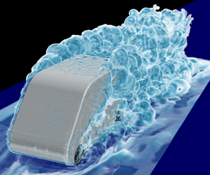
Figure 5 visualizes the instantaneous flow structures around the square-back van model predicted by resolved LES and the coarse PANS calculations from an axonometric perspective. The turbulent structures are presented using iso-surfaces of the second invariant of the velocity gradient (Q-criterion) with the value of Q = 1.5 × 10⁴ s⁻². The resolved LES can capture smaller eddies due to the well-repeating grid resolution. Nevertheless, the coarse PANS is able to capture the main separated flow near the A-pillars and in the wake region. Moreover, the separation mechanism and the evolution characteristics of the shear layer from small to larger eddies are well captured by both resolved LES and coarse PANS.

Figure 5. Iso-surfaces of Q-criterion with the value of Q = 1.5 × 10⁴ s⁻². (a) Resolved LES and (b) coarse PANS. Flow is from bottom left to top right in these images.

The flow structures observed near the lateral and lower trailing edges and the corresponding results of proper orthogonal decomposition (POD) and fast Fourier transform (FFT) analysis of the pressure field are shown in figures 6 and 7 for a better understanding of the capacity of PANS to predict the main flow structures and frequency. The methods for POD and FFT analysis have been readapted from the work of Minelli et al. (2017). For the POD and FFT analysis in the present study, the resolved LES data are taken as the baseline results, and the POD and FFT results of the coarse PANS results are then compared to the resolved LES. In the present study, the POD analysis is performed over 2880 snapshots for both resolved LES and the coarse PANS data. In both the resolved LES and the coarse PANS simulation, the snapshot data were extracted every twenty time steps from t^* = 114 to t^* = 266 (corresponding to approximately four flow passages through the domain), yielding a non-dimensional time interval between adjacent CFD snapshots of $\Delta t_{CFD}^\ast= \Delta {t_{CFD}}{U_{inf}}/W = 5.3 \times {10^{ - 2}}$. The comparisons of the POD and FFT results of the pressure fluctuation between the resolved LES and the coarse PANS are conducted in two interrogated domains. The horizontal interrogated domain I is placed near the lateral trailing edge with the height of z/W = 0.709, and its size is 0.97W (stream-wise direction) × 0.6W (span-wise direction), as depicted in figure 6(a,b). The vertical interrogated domain II is located downstream from the lower trailing edge with the span-wise coordinate of y/W = 0, and the size of the interrogated domain II is 0.47W (stream-wise direction) × 0.28W (vertical direction), as depicted in figure 7(a,b).

Figure 6. Comparison of the (c,d) most energetic pressure POD mode and (e, f) corresponding dominant frequency in the horizontal interrogated domain I between resolved LES (c,e) and coarse PANS (d, f). Panels (a) and (b) show the position and dimensions of the horizontal interrogated domain I. Flow is from left to right in these images.

Figure 7. Comparison of the (c,d) most energetic pressure POD mode and (e, f) corresponding dominant frequency field in the vertical interrogated domain II between resolved LES (c,e) and coarse PANS (d, f). Panels (a) and (b) show the position and dimensions of the vertical interrogated domain II. Flow is from left to right in these images.

Figure 6(c,d) presents the distribution characteristics of the coherent structures of the most energetic pressure POD mode extracted from the interrogated domain I. The coarse PANS captures similar features and spatial scales of the coherent structures of the most energetic pressure POD mode to the resolved LES, indicating that the coarse PANS can characterize the stream-wise pressure fluctuation inside the shear layers separated from the lateral trailing edges of the square-back van model. Figures 6(e) and 6( f) present the corresponding frequency of the most energetic pressure POD mode predicted by the resolved LES and the coarse PANS. It shows that the coarse PANS accurately predicts the dominant frequency $({F^ + } = 0.71)$ of the most energetic pressure POD mode, being the same as that of the resolved LES. Furthermore, the coarse PANS produces a smaller range of the dominant frequency, while the resolved LES has a broader distribution of the dominant frequency. This is because the coarse PANS only resolves the large-scale flow structures, avoiding the mixture of the multi-scale coherent structures, which contributes to a more significant behaviour of the simple harmonic motion of the time domain deduction, thus resulting into a filtering of the cross-contamination of frequencies in the pressure spectra.

To identify the accuracy of the coarse PANS in predicting the separation and evolution of the shear layer shedding from the lower trailing edge, figure 7 shows the comparison of the POD and FFT results of the pressure field in the interrogated domain II. Similar to the previous case, the coarse PANS is found to reproduce the features and evolution characteristics of the most energetic pressure POD mode found in the resolved LES. The dominant frequency of the most energetic pressure POD mode inside the interrogated domain II predicted by the coarse PANS is ${F^ + } = 1.01$, which is very close to that of the resolved LES $({F^ + } = 0.98)$. Moreover, the coarse PANS produces a similar spatial energy distribution to the resolved LES when the FFT analysis is conducted on ${F^ + } = 1.0$, indicating the high accuracy of the coarse PANS in predicting the main flow structures and frequencies in the wake region.

All of the results reported above indicate that the PANS method works well for the prediction of the turbulent flow structures around a square-back van model, which presents a significant advantage compared to the LES method when the grids adopted for the simulation are too coarse. Furthermore, the overall good agreement with the PIV experiments (aerodynamic drag, recirculation bubbles, velocity and stress distribution) and the resolved LES calculation (aerodynamic drag, recirculation bubbles, velocity profiles, stress distribution, POD and FFT results of the shear layers) allow us to select the PANS method and coarse-resolution mesh to proceed in a more in-depth analysis on the results.

3.2. Effects of the ground and wheel motion on the aerodynamic performance of the square-back van model

After a comprehensive validation of the PANS method, in this section, the coarse PANS will be used to investigate the influence of moving ground and rotating wheels on the aerodynamics of the square-back van model. In § 3.2, the same van's geometry and wind speed applied at the inlet are selected, yielding the same Reynolds number Re = 2.5 × 10⁵ as in § 3.1. Specifically, for systematic comparison and determination of the effect introduced by the ground motion and the wheel rotation, three cases with different ground and wheel motions are studied: (i) stationary ground with stationary wheels (SGSW); (ii) moving ground with stationary wheels (MGSW) and (iii) moving ground with rotating wheels (MGRW). In the SGSW case, the van model with stationary wheels is parked on the stationary ground, and these boundary conditions are always represented in the traditional wind tunnel test concerning vehicle aerodynamics. For the MGRW case, the van's wheels are kept steady while the ground starts to move at the same speed as that applied at the inlet. The MGSW case is chosen because the van model could be hung above the moving belt in certain advanced wind tunnel laboratories. In the MGRW case, the ground condition is the same as that in the MGSW case, where the wheels are rotating inside the wheelhouses and their linear velocity is kept the same as the moving ground, which represents the real condition of a van model running in the open air. Additionally, the boundary condition details for the three cases are summarized in table 4, in which the angular velocity of the rotating wheels and the speed of the moving ground are set according to the incoming flow speed.

Table 4. Boundary condition details of the ground and wheels for PANS simulations.

3.2.1. Aerodynamic forces and pressure distribution

The time-averaged drag and lift coefficients obtained from the three cases are reported in table 5. The ground motion has a significant impact on the drag coefficient, and the moving ground leads to a 5.85 % drag reduction when comparing the C_d values between the MGSW case and the SGSW case. Compared to the MGSW case, the MGRW case causes a slightly higher C_d value, and the rotating wheels increase the C_d value by approximately 1.25 %. This suggests that, in terms of the drag coefficient, the differences between the SGSW and MGRW cases is approximately 4.4 %. For the comparison of the aerodynamic lift forces, the SGSW and MGRW have the highest and lowest negative C_l value, respectively. Compared to the SGSW case, the negative C_l values in the MGSW and MGRW cases reduce by 10.3 % and 22.4 %, respectively. This is because the ground's motion and wheel's rotation significantly increase the flow momentum beneath the van model and thereby cause a lower pressure distribution. This first analysis reveals that the moving ground and rotating wheels have a strong impact on the lift coefficient, while the effect on the drag coefficient should be more limited. The mechanism of the effects of the moving ground and rotating wheels on the van's aerodynamic forces will be further revealed throughout the comprehensive analysis of the surface pressure distribution (§ 3.2.2), the turbulent wake structures (§ 3.2.3) and the wheels’ surrounding flow characteristics (§ 3.2.4).

Table 5. Comparison of the drag and lift coefficients of the square-back van model between different ground conditions.

Figure 8 compares the pressure coefficient distribution along four van's outlines along the span-wise coordinates y/W = 0, 0.14, 0.28 and 0.42 among the SGSW, MGSW and MGRW cases. The general observation in figure 8 is that the ground motion and wheel rotation drastically decreases the pressure distribution on the bottom surface of the square-back van model (from point b to point f), while its influence on the pressure distribution on the van's top surface is negligible (from point g to point a). This is because the ground motion eliminates the boundary layer development on the ground and wheel rotation increases the stream-wise flow energy, which increases the flow momentum and lowers the pressure distribution beneath the van model. Compared to the SGSW case, the pressure difference between the upper and bottom surface of the square-back van model gradually increases with the moving ground and the rotating wheels, which in turn contributes to a 10.3 % and 22.4 % reduction of lift coefficient in the MGSW and MGRW cases, respectively.

Figure 8. Comparison of pressure distribution on the front, top, back and bottom surfaces of the van model along various span-wise distance from the middle centre plane. (a) y/W = 0, (b) y/W = 0.14, (c) y/W = 0.28 and (d) x/W = 0.42. SGSW (red solid line), MGSW (orange solid line) and MGRW (cyan solid line).

It can be seen from figure 8 that the SGSW case shows the highest positive pressure distribution on the van's windward surface (from point f to point g), while the positive C_p values along the windward surface in the MGSW and MGRW cases are basically the same. This is because the blocking effect caused by the growing boundary layer along with the stationary ground forces airflow to impinge on the upper van's windward surface, resulting in a higher positive pressure distribution on the upper windward surface. The reason for this phenomenon can be found in the comparison of the stream-wise velocity profiles along the vertical and span-wise lines in front of the van model presented in figure 9. The vertical sampling lines on the Plane-V (y/W = 0) and the span-wise sampling lines on the Plane-H (z/W = 0.365) are located at 0.25W, 0.5W, 0.75W and 1.0W upstream from the van's nose. It can be seen from figure 9 that for the stream-wise velocity distribution in the range from z/W = 0 (ground height) to z/W = 0.118 (van's bottom height), the SGSW case shows a lower value of stream-wise velocity than the MGSW and the MGRW cases, owing to the growing boundary layer along with the stationary ground. As the sampling position exceeds z/W = 0.118, the SGSW case presents a higher stream-wise velocity than the MGSW and the MGRW cases, thereby resulting in a stronger impingement on the van's windward surface, which well explains the positive pressure difference on the windward surface in three cases presented in figure 8. Additionally, the stream-wise velocity distribution in front of the van model shows good agreement in the MGSW and the MGRW cases, indicating a negligible influence of wheel rotation on the flow characteristics upstream the van model under moving ground condition.

Figure 9. Comparison of the stream-wise velocity profiles with the upstream distance of 0.25W, 0.5W, 0.75W and 1.0W from the van's nose on the (a) horizontal Plane-H with the z coordinate of y/W = 0.365 and the (b) vertical Plane-V with the span-wise coordinate of y/W = 0.

For a quantitative analysis of the ground and wheel motion on the aerodynamic drag of the van body, the pressure drag coefficient $({C_{d - P}})$ has been computed by the normalized stream-wise pressure integration on the integral surfaces, defined as ${C_{d - P}} = \int\!\!\!\int_s {\overline {{P_x}} \,\textrm{d}s} /(0.5\rho U_{inf}^2S)$, with $\int\!\!\!\int_s {\overline {{P_x}} \;\textrm{d}s}$ being the integral of the stream-wise pressure force acting on the integral surfaces and $0.5\rho U_{inf}^2S$ being the reference dynamic pressure force. Note that the positive ${C_{d - p}}$ value means the direction of the pressure drag coefficient acting on the van's integral surface is the same as the incoming flow direction. The ${C_{d - p}}$ values on the windward and leeward surfaces of the carbody in the SGSW, MGSW and MGRW cases are calculated and compared in figure 10. The windward and leeward pressure integral surfaces (IS-1 and IS-2) of the carbody are highlighted by the red lines in figure 10(a). The h-i-j-k and h’-i’-j’-k’ curves represent the windward (IS-1) and leeward (IS-2) pressure integral surfaces, respectively.

Figure 10. Comparison of the pressure drag coefficient calculated by the normalized stream-wise pressure integration of the carbody in SGSW, MGSW and MGRW cases. (a) The surfaces used to perform the integrals on the carbody, wheels and wheelhouses. IS-1, IS-3 and IS-5 (IS-2, IS-4 and IS-6) represent the windward (leeward) integral surfaces of the carbody, wheels and wheelhouses. (b) Comparison of the pressure drag coefficients of the IS-1, IS-2 and IS-1 + IS-2.

Figure 10(b) shows that the ${C_{d - P}}$ value computed on the IS-1 is the highest in the SGSW case, while there is no difference between the MGSW and the MGRW cases, which yield the same ${C_{d - P}}$ values, 15.9 % lower than the SGSW case. This is because the moving ground eliminates the boundary layer effects and thereby relieves the impingement on the IS-1 caused by the impending airflow, as depicted in figures 8 and 9. In contrast, the ${C_{d - P}}$ value computed on the IS-2 shows a dependence on the investigated case, with the SGSW and the MGRW cases yielding the lowest and the highest ${C_{d - P}}$ values, respectively. In particular, compared to the SGSW case, the ${C_{d - P}}$ value computed on the IS-2 in the MGSW and MGRW cases increases by approximately 2.2 % and 3.5 %, respectively. The reason for this phenomenon is that the SGSW case is characterized by higher values of the pressure on the base than that in the MGSW and MGRW cases, and the effects of the rotating wheels result in lower C_p values than those attained in the MGSW case (as shown in figure 8). Finally, the ${C_{d - P}}$ value computed on IS-1 + IS-2 shows that the case that is characterized by the lowest value of ${C_{d - P}}$ is the MGSW, although this value is only 0.8 % less than the MGRW case. However, the SGSW case shows an overestimate of the drag coefficient with respect to the more realistic configurations of MGRW of approximately 5 %. These results are in good agreement with the observation listed in table 5.

3.2.2. Turbulent wake structure

Figure 11 reports the 2-D streamlines overlaid to the contour maps of the time-averaged stream-wise velocity for the SGSW, MGSW and MGRW cases. The vertical plane is located on the middle centre plane of the square-back van model in the span-wise direction (y/W = 0). The general finding in figure 11 is that the ground and wheel motion greatly influence the vortex core positions of A and B. The ground motion contributes to the 4.83 % upward movement of the vortex A core and 21.82 % downward movement of vortex B, indicating a larger impact of ground motion on the lower bubble, when comparing the MGSW case with the SGSW case. Compared to the MGSW case, the wheel rotation shortens the distance of the vortex B core from the lower rear base. In contrast, the distance of the vortex A core from the upper rear base in the MGRW case remains the same as in the MGSW case, resulting in lower pressure values on the lower rear base than in the MGRW cases (presented in figure 8), which is one of the reasons why the rotating wheels increase the aerodynamic drag force of the square-back van model under the moving ground condition. However, the motion of the ground and the wheels does not significantly influence the length of the vertical planar recirculation region, while it affects the configuration of the recirculation region. In particular, figure 11(d) shows an upward shift of the recirculation region by the ground motion. The ground motion and wheel rotation dramatically change the coordinates of the saddle point on the vertical plane (S_V). Compared to the SGSW case, the coordinates of S_V in the MGSW case displace by 16.82 % and 50.72 % in the x and z direction, while the stream-wise and vertical coordinates of S_V in the MGRW case increase by 7.63 % and 41.89 %, respectively. Because the saddle point locates on the boundary of two adjacent vortices, where the flow field is unstable accompanied with strong fluctuation of the velocity, and the significant influence of the moving ground and rotating wheels on the saddle point will certainly affect the distribution characteristics of the Reynolds stress and the turbulence kinetic energy in the wake region.

Figure 11. Comparison of averaged planar velocity magnitude u/U_inf contour overlaid with 2-D streamlines on the symmetrical plane y/W = 0. (a) SGSW, (b) MGSW, (c) MGRW. The red upper triangle (upper vortex centre), red lower triangle (lower vortex centre), red square (saddle point). (d) Comparison of the positions of the vortex centre and saddle point, and vertical planar recirculation region. SGSW (orange colour), MGSW (yellow colour), MGRW (cyan colour). Flow is from left to right in these images. SGSW (orange solid line).

The dominant effects of the ground and wheel motion on the near wake structures can also be observed from the mean stream-wise velocity contour on the horizontal plane in figure 12. The horizontal plane is located at the middle height of the rear base of the van model in the vertical direction (z/W = 0.51). Compared to the SGSW case, the ground motion and the wheel rotation gradually compress the horizontal planar recirculation region, contributing to the longest and the shortest length of the horizontal planar recirculation region in the SGSW and MGRW cases, which thereby causes the highest and the lowest C_p value distribution in the SGSW and MGRW cases presented in figure 8. Although the SGSW case has a higher base pressure distribution than the other two cases, the stronger impingement on the windward surface in the SGSW cases results in the largest van's pressure drag of the three cases. Specifically, the MGRW case has a shorter distance of the vortices C and D cores from the rear base than that in the MGSW case, which explains why the rotating wheels increase the aerodynamic drag of the square-back van model.

Figure 12. Comparison of averaged planar velocity magnitude u/U_inf contour overlaid with 2-D streamlines on the horizontal plane z/W = 0.51. (a) SGSW, (b) MGSW, (c) MGRW. The red triangles (vortex centre), red square and circle (saddle point). The red upper triangle (upper vortex centre), red lower triangle (lower vortex centre), red square (saddle point). (d) Comparison of the positions of the vortex centre and saddle point, and horizontal planar recirculation region. SGSW (orange colour), MGSW (yellow colour), MGRW (cyan colour). Flow is from left to right in these images. SGSW (orange solid line).

Moreover, the ground and wheel motions greatly affect the position of the saddle points on the horizontal plane (S_H). For the SGSW case, a pair of saddle points (S_{H -1} and S_{H -2}) on the horizontal plane are noticeable, being symmetric about the middle centre plane (y/W = 0). Both the moving ground and the rotating wheel cases force S_{H -1} and S_{H -2} to merge at the symmetry plane. The configuration of the pair of stream-wise vortices (E and F) generated by the roll-up of the wake detaching from the corners of the upper trailing edge are presented in figure 13 for the three investigated cases. As the ground moves, the vortices E and F move inward in the span-wise direction, and the span-wise distance between vortices E and F in the MGSW case decreases by 7.06 % compared to that in the SGSW case. The rotating wheels are found to result in a 3.97 % increase of the span-wise distance between the vortices E and F cores and a 3.26 % increase of the vertical distance of the vortices E and F cores from the ground under moving ground conditions. Additionally, a pair of vortices (G and H) shedding from the front wheels are clearly visible for the SGSW case, while they disappear in the MGSW and MGRW cases owing to the ground motion.

Figure 13. Comparison of averaged planar velocity magnitude u/U_inf contour overlaid with 2-D streamlines on the vertical plane x/W = 0.4. (a) SGSW, (b) MGSW, (c) MGRW. The red square (vortex centre behind van back), red cross (vortex centre near the ground). (d) Comparison of the positions of the vortex centre. SGSW (orange colour), MGSW (yellow colour), MGRW (cyan colour).

In figure 14, the growth characteristics of the shear layers separated from the left and lower trailing edges are analysed in detail to check the effects on the turbulent wake flow induced by the ground and wheel motion. The growth of the left and lower shear layers is characterized by the vorticity thickness defined by

Figure 14. Comparison of the growth characteristics of the shear layers separated from the rear trailing edges of the square-back van model. (a) Left shear layer growth characteristic, (b) lower shear layer growth characteristic. SGSW (orange colour), MGSW (yellow colour), MGRW (cyan colour). The vertical dashed lines represent the planar recirculation region length. Flow is from left to right in these images.

(3.3)\begin{gather}\delta (\omega ,y) = \frac{{{U_{max}} - {U_{min}}}}{{ma{x_{[y]}}\left[ {\frac{{\partial u(x,y,z)}}{{\partial y}}} \right]}},\end{gather}

(3.4)\begin{gather}\delta (\omega ,z) = \frac{{{U_{max}} - {U_{min}}}}{{ma{x_{[z]}}\left[ {\frac{{\partial u(x,y,z)}}{{\partial z}}} \right]}}.\end{gather}

Figure 14(a,b) presents the distribution of $\delta (\omega ,y)/W$ of the left shear layer on the z/W = 0.709 horizontal plane and $\delta (\omega ,z)/W$ of the lower shear layer on the y/W = 0 vertical plane. For the distribution of $\delta (\omega ,y)/W$ within two lateral shear layers, the vorticity thickness difference between three cases is clearly observed in the region from x/W = 0.4 to x/W = 1.2, as shown in figure 14(a), and the growth rates in the three cases are similar. In particular, the MGRW and SGSW cases have the thickest and the thinnest lateral shear layer, contributing to the shortest and the longest horizontal planar recirculation region length in the MGRW and SGSW cases, which well explains the increasing ${C_{d - P}}$ value of the rotating wheels under the moving ground condition. As depicted in figure 14(b), the $\delta (\omega ,z)/W$ distribution of the lower shear layer on the y/W = 0 vertical plane in the three cases presents the same behaviour. In particular, $\delta (\omega ,z)/W$ increases from x/W = 0 to x/W = 1.0, then it gradually decreases from x/W = 1.0 to x/W = 2.0. The MGSW and MGRW cases have the similar growth rate from x/W = 0 to x/W = 1.0, while the growth rate of the SGSW case is lower than the MGSW and MGRW cases. Focusing on the behaviour of $\delta (\omega ,z)/W$ (from x/W = 0 to x/W = 1.0), the MGRW case is characterized by a thicker lateral shear layer than the MGSW. This is associated with the reduced values of C_p in the rotating wheel case, thereby leading to an increase in the van's pressure drag. Additionally, although the SGSW case shows the thinnest lateral and lower shear layers, the SGSW case features the highest drag value due to the greater pressure values on the windward surface.

Figure 15 compares the stream-wise and vertical velocity component profiles in the middle centre plane y/W = 0. The velocity profiles are measured at three different stream-wise locations: x/W = 0.25, 0.5 and 0.75. The general finding from figure 15(a–c) is that the ground motion and wheel rotation mainly influence the stream-wise velocity distribution within the lower part of the wake region (from z = 0W to z = 0.5W), and ground motion has a more considerable impact on u profiles than that induced by the wheel rotation. The difference in u profiles among the three cases becomes more significant with the increasing stream-wise distance between the rear base and the profiles. In particular, for the comparison in figure 15(a), u profiles are different only up to approximately z = 0.12W, which is the position of the shear layer from the underbody. Moreover, the moving ground is found to significantly increase the stream-wise velocity distribution in the wake region due to the increasing momentum near the ground. This also results in a cross of u profiles in the lower part of the wake region, showing good agreement with the wake comparison of a slanted back Ahmed body between the stationary and moving ground (Krajnović & Davidson 2005). Furthermore, the rotating wheels slightly increase the stream-wise velocity distribution in the wake region compared to the MGRW case to the MGSW case, showing good consistency with the observation reported by Wang et al. (2020). The averaged vertical velocity profiles in the symmetrical plane (y/W = 0) of the square-back van model are also compared for the three cases. The general observation in figure 15(d–f) is that the ground motion and the wheel rotation play an essential role in altering the vertical velocity distribution in the wake region. The vertical velocity difference among the three cases becomes more evident with the increasing distance of the profiles from the rear base. Different from the u profile comparison shown in figure 15(a–c), the motion of the ground and wheels not only dramatically changes the vertical velocity distribution in the lower wake region but also in the upper wake region (see figure 15d–f), indicating a global effect of moving ground and rotating wheels on the velocity distribution in the wake flow.

Figure 15. (a–c) Averaged stream-wise and (d–f) vertical velocity components at different locations along the recirculation bubble in the symmetrical plane (y/W = 0) in the near wake: (a,d) x ₁/W = 0.4; (b, e) x ₂/W = 0.8; (c, f) x ₃/W = 1.2. SGSW (grey solid line), MGSW (dark grey dashed line), MGRW (black solid line). Flow is from left to right in these images.

The dominant effect of the moving ground and rotating wheels on the near wake flow can be observed from the stream-wise and vertical normal stress components ($\overline {u^{\prime}u^{\prime}} /U_{inf}^2$ and $\overline {w^{\prime}w^{\prime}} /U_{inf}^2$) and the vertical planar turbulence kinetic energy ${k_{xz}} = 0.5 \times (\overline {u^{\prime}u^{\prime}} /U_{inf}^2 + \overline {w^{\prime}w^{\prime}} /U_{inf}^2)$ on the symmetrical plane (y/W = 0) in figure 16. The moving ground has a significant impact on the distribution characteristics of the normal stress components and the vertical planar turbulence kinetic energy in the lower wake region and the upper wake region, confirming the global effect of the ground condition again. As evidenced in figure 16, the shear layer separating from the lower trailing edge is observed to be inclined upward in the SGSW case. In contrast, this lower shear layer deflects towards the ground in the MGSW and MGRW cases, owing to the increasing flow momentum of the underbody flow brought by the moving ground. Moreover, it can be seen from figure 16(a), the lower shear layer presented by stream-wise normal stress in the SGSW case interferes with the turbulent flow separated from the stationary ground. However, this phenomenon disappears immediately in the MGSW and MGRW cases. Compared to the MGSW case, the rotating wheels in the MGRW case contribute to a lower turbulence intensity on the symmetric plane. This is because the rotating wheels force more airflow between two-side wheels in the lower wake region to flow towards the wheel wake, thereby decreasing the velocity fluctuation energy in the middle wake.

Figure 16. Comparison of (a) averaged normal stress $\overline {u^{\prime}u^{\prime}} /U_{inf}^2$, (b) $\overline {w^{\prime}w^{\prime}} /U_{inf}^2$ and (c) planar turbulence kinetic energy k_xy on the symmetrical plane y/W = 0 between SGSW (left), MGSW (middle) and MGRW (right). Flow is from left to right in these images.

Figure 17 visualizes the stream-wise and span-wise normal stress components ($\overline {u^{\prime}u^{\prime}} /U_{inf}^2$ and $\overline {v^{\prime}v^{\prime}} /U_{inf}^2$) as well as the horizontal planar turbulence kinetic energy ${k_{xy}} = 0.5 \times (\overline {u^{\prime}u^{\prime}} /U_{inf}^2 + \overline {v^{\prime}v^{\prime}} /U_{inf}^2)$ on the middle height of the rear base in the vertical direction (z/W = 0.51). The general finding in figure 17 is that the fluctuation intensity of the stream-wise and span-wise velocity components on the horizontal plane becomes higher in the moving ground cases, thereby contributing to the larger scale of the lateral shear layers compared to that in the SGSW case. Furthermore, figure 17(b) shows that the MGRW case produces a higher level of the span-wise normal stress on the horizontal plane than that in the MGSW case, owing to the driving effect of rotating wheels on the lower wake flow in the span-wise direction. Additionally, figure 18 compares the stream-wise normal stress distribution characteristics on the vertical plane with the stream-wise distance of x/W = 0.4 from the rear base. The moving ground evidently influences the fluctuation intensity in the lower and lateral shear layers while presenting less impact on the upper shear layer. In particular, the moving ground mainly strengthens the velocity fluctuation near the lower trailing edge of the square-back van model, while the rotating wheels primarily evacuate the velocity fluctuation in the middle wake region towards the wheel wake region.

Figure 17. Comparison of (a) averaged normal stress $\overline {u^{\prime}u^{\prime}} /U_{inf}^2$, (b) $\overline {w^{\prime}w^{\prime}} /U_{inf}^2$ and (c) planar turbulence kinetic energy k_xy on the horizontal plane z/W = 0.51 between SGSW (left), MGSW (middle) and MGRW (right). Flow is from left to right in these images.

Figure 18. Comparison of (a) averaged normal stress $\overline {u^{\prime}u^{\prime}} /U_{inf}^2$, (b) $\overline {w^{\prime}w^{\prime}} /U_{inf}^2$ and (c) planar turbulence kinetic energy k_xy on the vertical plane x/W = 0.4 between SGSW (a), MGSW (b) and MGRW (c).

3.2.3. Flow characteristics around the wheels

Figure 19 compares the 3-D time-averaged iso-surfaces of Q-criterion with the value of Q = 5 × 10² s⁻² between the SGSW, MGSW and MGRW cases, and the 3-D time-averaged Q-criterion is coloured by the normalized mean stream-wise vorticity $\omega _x^\ast= \omega \cdot W/{U_{inf}}$. The general finding in figure 19 is that the distribution characteristics of the vortex structures is significantly affected by the ground motion. In particular, the ground vortex structures ahead and downstream of the van body are clearly visible in the SGSW case, because of the boundary layer effect of the stationary ground, and these ground vortex structures disappear as the ground starts to move (MGSW and MGRW cases). In addition, the longitudinal vortex structures separated from the front wheelhouse in the SGSW case are much longer than those in the MGSW and MGRW cases, and the size and strength are significantly enhanced by the rotating wheels, reasonably explaining the larger van's aerodynamic drag in the MGRW than in the MGSW case and the observation of vortices E and F of the SGSW case in figure 13. Furthermore, the wheel rotation not only enhances the vortex separation near the front wheelhouse and on the rear wheel surface, but also enlarges the vortex structures separated from the A-pillar, when comparing the 3-D time-averaged Q-criterion between the MGSW and MGRW cases, that is the reason why the wheel rotation increases the van's aerodynamic drag under the circumstance of the moving ground.

Figure 19. Comparison of the 3-D time-averaged iso-surfaces of Q-criterion with the value of Q = 5 × 10² s⁻². (a) SGSW, (b) MGSW, (c) MGRW. The 3-D time-averaged Q-criterion is coloured by the mean stream-wise vorticity. Flow is from top left to bottom right in these images.

Figure 20 compares the flow structures around the front wheelhouse in the SGSW, MGSW and MGRW cases. The flow features around the front wheelhouse and the A-pillars are captured by the horizontal and vertical planes coloured by the span-wise velocity component (v/U_inf). The planar vortex structures on the vertical and horizontal planes are coloured using the normalized mean vertical and stream-wise vorticity, in which the vortex cores of the recirculation bubbles separated from the A-pillars and front wheelhouse are denoted using the black plus sign (V_{A -1} and V_{A -2}) and white plus sign (V_{W -1} and V_{W -2}). The planar vortex structures on the vertical and horizontal planes are coloured using the normalized mean vertical and stream-wise vorticity. For a more intuitive visualization, the stagnation points, separation and reattachment lines of the A-pillar, and separation and reattachment lines of the front wheelhouse are presented using dash–dot cyan line, dash green line, dash pink line, solid green line and pink solid line, respectively. An interesting observation in figure 20, evidenced by the streamlines, is that the air flows into the front wheelhouse from the rear gap and flows upstream inside the upper front wheelhouse, then streamlines flow out of the wheelhouse from the front gap and interfere with the recirculation bubble separated from the A-pillars. The moving ground and rotating wheels affect the flow separation and reattachment at the front wheelhouse, thereby changing the flow separation and corresponding reattachment caused by the A-pillars.

Figure 20. Comparison of the flow structures around the front wheelhouse between the SGSW, MGSW and MGRW cases. The van body and wheels are coloured by the time-averaged C_p overlaid with the surface streamlines. The flow characteristics around the front wheelhouse and A-pillars are captured by the horizontal and vertical planes coloured by the span-wise velocity component. The planar vortex structures on the vertical and horizontal planes are coloured using the normalized mean vertical and stream-wise vorticity. The vortex cores of the recirculation bubbles separated from the A-pillars and front wheelhouse are denoted using the black plus sign (V_{A -1} and V_{A -2}) and white plus sign (V_{W -1} and V_{W -2}). The stagnation points, separation and reattachment lines of the A-pillar, and separation and reattachment lines of the front wheelhouse are presented using dash–dot cyan line, green dash line, dash pink line, solid green line and solid pink line. Flow is from bottom left to top right in these images.

Table 6 compares the coordinates of the pressure stagnation point and the vortex cores (V_{A -1}, V_{A -1}, V_{W -1} and V_{W -2}) for the quantitative analysis of the ground and wheel motion effects on the separation flow around the A-pillars and front wheelhouse. It can be seen from table 6 that the height of the pressure stagnation point significantly decreases by 5.4 % as the ground starts to move, while the wheel rotation has a negligible influence on the height of the pressure stagnation point under the moving ground condition. Furthermore, comparing the front wheelhouse vortex core position (V_{W -1} and V_{W -2}) in the MGRW case to the MGSW case, the vertical coordinate of the vortex V_{W -1} core moves upward by 8 % and the stream-wise coordinate of the vortex V_{W -2} core moves forward by 2.2 %, respectively. The movement of the vortex V_{W -1} and V_{W -2} cores toward the A-pillars forces the vortex V_{A -1} and V_{A -2} cores to move away from the van body, contributing to a larger recirculation bubble separated from the A-pillar, which is the second reason why the rotating wheels result in higher aerodynamic drag under the moving ground condition.

Table 6. Comparison of the coordinates of the stagnation point on the windward surface and the vortex cores around the front wheelhouse.

Figure 21 compares the flow structures aside and behind the rear wheelhouse among the SGSW, MGSW and MGRW cases. Three vertical planes are used to present the flow characteristics around the rear wheelhouse. The 2-D streamlines are plotted and the rear wheels are coloured using the time-averaged C_p value for a more intuitive visualization. The general finding in figure 21 is that the size of the vortex G is the largest in the SGSW case and smallest in the MGRW case, showing good agreement with the observation in figure 19. In figure 21, the pressure iso-surface with the value of C_p = −0.5 is used to present the wake topology of the rear wheels. A pair of longitudinal vortices (Lⁱⁿ and L^out) separated from the predestined ties of the rear wheels are clearly visible. In particular, the length and size of the Lⁱⁿ and L^out are the smallest under the stationary ground condition. As the ground begins to move, the increasing underbody flow momentum enhances the separating strength of Lⁱⁿ and L^out. Moreover, compared to the MGSW case, the kinetic energy input induced by the wheel rotation in the MGRW case elongates and enlarges the Lⁱⁿ and L^out, thereby contributing to the higher ${C_{d - P}}$ value of the rear wheels.

Figure 21. Flow structures behind and aside the rear wheelhouse in the SGSW, MGSW and MGRW cases. The rear wheels are coloured using the time-averaged C_p. The longitudinal vortex structures separated from the windward and leeward surface of the rear wheel are presented using the static pressure iso-surface with the value of C_p = −0.5. The planar vortex structures on three sampling planes are coloured by normalized stream-wise vorticity. Flow is from up left to bottom right in these images.

Figure 22 compares the pressure drag coefficients of the wheelhouses (${C_{d - P}}$ value of IS-3 + IS-4) and wheels (${C_{d - P}}$ value of IS-5 + IS-6) in the SGSW, MGSW and MGRW cases. The windward and leeward surfaces used for the pressure integration on the wheelhouses (IS-3 and IS-4) and wheels (IS-5 and IS-6) are marked in figure 10(a), in which l-m-n-o and l’-m’-n’-o’ represent the windward (IS-3) and leeward (IS-4) pressure integral surfaces of the wheelhouse, respectively. Similarly, p-q-r-s and p’-q’-r’-s’ represent the windward (IS-5) and leeward (IS-6) surfaces of the wheels, respectively. Moreover, FLWH, FRWH, RLWH and FRWH in figure 22(a) represent the left front, right front, left rear and right rear wheelhouses, and the FLW, FRW, RLW and FRW in figure 22(b) mean the left front, right front, left rear and right rear wheels (highlighted in figure 10a). The general finding in figure 22 is that the ground motion and the wheel rotation increase the ${C_{d - P}}$ values of the wheelhouses and the wheels. In particular, compared to the MGSW case, the rotating wheels increase the wheels’ total ${C_{d - P}}$ value by approximately 8 %. This is addressed to the fact that the rotating wheels generate a much more significant separated wake around the wheels, as it is shown in figure 21. Furthermore, compared to the MGSW case, the rotating wheels in the MGRW case increase the ${C_{d - P}}$ values of the front and rear wheelhouses by approximately 15 % and 56 %, respectively. This is mainly because the wheels’ rotation forces more airflow to impinge on the IS-4 of the wheelhouses, thereby increasing the total ${C_{d - P}}$ values of the four wheelhouses, which is the third reason why the rotating wheels increase the van's aerodynamic drag under the moving ground condition.

Figure 22. Comparison of the pressure drag coefficients of the wheelhouses and the wheels in the SGSW, MGSW and MGRW cases. Integral of the normalized stream-wise pressure of the (a) four wheels and (b) wheelhouses. FLW, FRW, RLW and FRW represent the left front, right front, left rear and right rear wheels (refer to figure 10a). FLWH, FRWH, RLWH and FRWH represent the left front, right front, left rear and right rear wheelhouses (refer to figure 10a).

Figure 23 compares the stream-wise underbody flow rate and the normal stress distribution behind the rear wheel between the SGSW, MGSW and MGRW cases. The normalized flow rate $F_r^\ast $ is defined as $F_r^\ast= \int\!\!\!\int_s {\bar{u}\,\textrm{d}s} /({U_{inf}}S)$, thus representing the ratio of the integral value of the stream-wise velocity on the vertical sampling plane $(\int\!\!\!\int_s {\bar{u}\,\textrm{d}s} )$ to the reference flow rate $({U_{inf}}S)$. The moving ground significantly increases the flow rate in the vicinity of the ground owing to the cancellation of the boundary layer developing on the ground. Furthermore, compared to the MGSW case, the flow rate distribution behind the rear wheelhouse in the MGRW case decreases obviously, indicating a larger velocity loss in the near wake region of the rear wheels. This is because the rotating wheels increase the vertical kinetic energy while decreasing the stream-wise component. Moreover, compared to the SGSW case, the ground motion and wheel rotation gradually increase the stream-wise normal stress level both inside and outside the rear wheels due to the larger scale of the Lⁱⁿ and L^out vortices. Additionally, compared to the MGSW case, the $\overline {u^{\prime}u^{\prime}} /U_{inf}^2$ value near the lateral diffuser in the MGRW case significantly increases, showing good agreement with the local C_p iso-surface distribution presented in figure 21, which can be attributed to another reason why the rotating wheels increase the van's drag value under the moving ground condition.

Figure 23. Comparison of the stream-wise underbody flow rate and the normal stress distribution behind the rear wheel between the SGSW, MGSW and MGRW cases. (a) Stream-wise flow rate distribution and (b) stream-wise normal stress distribution. The red vertical lines indicate the wheels’ wake range with the span-wise coordinates of y/W = ± 0.25.

3.2.4. POD and FFT analyses of the wake shear layers

This section explores the effects of the moving ground and rotating wheels on the most energetic pressure POD mode and its corresponding dominant frequency, to identify whether the moving ground and the rotating wheel conditions need to be reproduced when performing analysis of the turbulent wake characteristics for a square-back van model in a wind tunnel. Note that the dominant frequencies of the SGSW, MGSW and MGRW cases in figures 24 and 25 are normalized using ${F^\ast } = f \cdot {L_r}/{U_{inf}}$, where L_r is the corresponding vertical planar recirculation region length highlighted in figure 11, and f represents the frequency in Hertz. Figures 24(c) and 24(d) compare the spatial distribution of the coherent structures of the most energetic pressure POD mode in the horizontal interrogated domain I for the three investigated cases. The moving ground primarily affects the length scales of the coherent structures rather than the distribution characteristics in the horizontal interrogated domain I. Conversely, the same length scales are found to be unaffected by the rotating wheels in the MGRW case, when compared to the MGSW case. The dominant frequencies in the MGSW case and the MGRW case are found to decrease to ${F^\ast } = 0.50$ and ${F^\ast } = 0.52$, respectively, with respect to the SGSW case $({F^\ast } = 0.58)$. This indicates a dominant effect of the moving ground on decreasing the shedding frequency of the shear layers near the lateral trailing edges.

Figure 24. Comparison of the (a–c) most energetic pressure POD mode and (d–f) corresponding dominant frequency in the horizontal interrogated domain I among SGSW (left), MGSW (middle) and MGRW (right). Refer to figures 6(a) and 6(b) for the position of the horizontal interrogated domain I. Flow is from left to right in these images.

Figure 25. Comparison of the (a–c) most energetic pressure POD mode and (d–f) corresponding dominant frequency in the vertical interrogated domain II among SGSW (left), MGSW (middle) and MGRW (right). Refer to figures 7(a) and 7(b) for the position of the vertical interrogated domain II. Flow is from left to right in these images.

Figure 25(a–c) compares the spatial distribution of the coherent structures of the most energetic pressure POD mode in the vertical interrogated domain II for the three investigated cases. The moving ground is found to significantly affect the evolution characteristics of the shear layer shedding from the lower trailing edge. In the SGSW case, the coherent structures evolve along an upward direction, which instead becomes a downward inclination in the moving ground cases because of the increasing underbody flow speed in the near wake region (see figure 15a–c). Furthermore, the moving ground and the rotating wheels dramatically increase the spatial scales of the coherent structures inside the lower shear layer, with a corresponding reduction of the normalized frequency. Indeed, figure 25(d–f) shows the dominant effect of the moving ground and the rotating wheels on the corresponding dominant frequency of the most energetic pressure POD mode in the vertical interrogated domain II. The moving ground decreases the corresponding dominant frequency to ${F^\ast } = 0.42$ (MGSW case) from ${F^\ast } = 0.83$ (SGSW case). As the wheels start to rotate, the corresponding dominant frequency increases again to ${F^\ast } = 0.61$ (MGRW case) compared to that in the MGSW case. The highlighted effects of the ground and the wheel motion on the dominant frequency, evolution and development characteristics of the wake shear layers suggest the need to reproduce the ground and wheels motion when conducting experimental studies on the van's turbulent wake characteristics. This is often at odds with the constraints imposed by the available equipment, as well as with the significant complication of the test section to introduce the moving ground. It is therefore of great importance to mitigate the effects of the boundary layer growth on the ground, which is found to be responsible for a great number of differences when investigating the wake dynamics.

4. Conclusion

In this paper, PANS simulations, at Re = 2.5 × 10⁵, were conducted to investigate the effect of the moving ground and rotating wheels on the aerodynamic behaviours of a square-back van model. In the first part of the paper, the PANS approach was validated against the wind tunnel experiments and the resolved LES under the circumstance of stationary ground, showing the potential of capturing the main flow features, even with a coarse mesh, far from being resolved for LES. In particular, a fine grid of 33 million elements was used to perform the resolved LES simulation, while a much coarser grid of 12 million elements was employed to conduct the coarse PANS calculation. The comparison of the aerodynamic drag value between the PANS, LES and the experiment is conducted. The averaged flow velocity and shear stress are also compared in the observed domain region. Furthermore, the validation involved modal and frequency analyses by means of POD and FFT, respectively. The pressure field in both horizontal and vertical interrogated domains, sampled in the numerical simulations only, was compared between PANS and LES, showing a good agreement by the structures and frequencies observed in both POD and FFT analysis. Finally, the predicting accuracy and computational costs of the LES and PANS methods with different grid resolutions were compared, and the PANS method using a low-resolution grid was found to present similar results to the resolved LES with an approximately 9 % CPU hour reduction. Overall, the validation demonstrates a better prediction by PANS when a drastically coarser grid is used and a good prediction of the main important structures and frequencies of the flow field.

After the validation process with a comparison with experimental data at the same Reynolds number and on the same geometry, in the second part of the study, the PANS method with a coarse grid of 12 million elements is used to investigate the effects of moving ground and rotating wheels on the aerodynamic behaviours of the square-back van model. The aerodynamic drag and lift forces are compared between the SGSW (stationary ground and stationary wheels), MGSW (moving ground and stationary wheels) and MGRW (moving ground and rotating wheels) cases. Compared to the stationary ground condition (SGSW), the drag value is found to decrease by 5.85 % in the MGSW case as a consequence of the underbody flow rate variation and the downward movement of the pressure stagnation point on the windward surface brought by the disappearing boundary layer on the ground, which thereby decreases the stream-wise normalized pressure integration on the windward surface (${C_{d - P}}$ value of IS-1) and the total pressure drag in the MGSW case. Moreover, based on the moving ground condition, the rotating wheels increase the van's aerodynamics drag, and the mechanism for this can be summarized by three points. On the one hand, the rotating wheels increase the vorticity thickness of the shear layers separated from the rear trailing edges, contributing to a shorter distance of the planar vortex cores on the vertical (vortices A and B) and horizontal (vortices C and D) planes from the rear base, and thereby cause lower pressure distribution on the rear base and contribute to higher pressure drag. On the other hand, the rotating wheels change the separation and reattachment characteristics near the front wheelhouse, which contributes to the larger longitudinal vortices separated from the front wheelhouse and the recirculation bubble separated from the A-pillars, thus resulting in larger aerodynamic drag of the van body. In addition, the rotating wheels enlarge the pairs of the longitudinal vortices (Lⁱⁿ and L^out) separated from the predestined ties of the wheels and increase the total ${C_{d - P}}$ value of the wheels by approximately 8 %. Furthermore, the rotating wheels forces more airflow to impinge on the IS-4 of the wheelhouses, and thereby increases the ${C_{d - P}}$ values of the front and rear wheelhouses by approximately 15 % and 56 %, respectively. Simultaneously, the ground motion and wheel rotation also contribute to an increased bottom surface pressure and unchanged upper surface pressure, contributing to the increased underbody flow momentum brought by the moving ground and the rotating wheels. This thereby decreases the lift force by 10.28 % in the MGSW case and 22.43 % in the MGRW cases when compared to that in the SGSW case.

Additionally, the moving ground and rotating wheels have a large impact on the flow structures and the velocity profiles in the wake behind the square-back van model. The difference in the wake flow is limited primarily to the region in the vicinity of the lower shear layer coming from the underbody of the vehicle. Furthermore, the ground motion is found to have a larger impact on the Reynolds stress on the turbulent kinetic energy in the lower wake region while having limited influence on the upper wake region. The moving ground alters the flow direction of the lower shear layer from an upward inclination to a downward inclination and strengthens the velocity fluctuation in the wake region. Based on the moving ground condition, the rotating wheels decrease the Reynolds stress and the turbulent kinetic energy in the middle wake region while increasing those in the wheel wake region. Finally, the evolution characteristics of the shear layers shedding from the lower and lateral trailing edges and the corresponding dominant frequencies of the most energetic pressure POD mode are found to be substantially different in the SGSW, MGSW and MGRW cases, which thereby dramatically affects a potential actuation signals. Based on the discussion above, we conclude that there are clear indications of the influence of the moving status of the vehicle and wheels on the aerodynamic forces, the recirculation bubbles, velocity profiles, Reynolds stress and turbulent kinetic energy in the wake region, and the distribution characteristics of the shear layers in the spatial and temporal domain. Thus, the relative motion between the ground, the vehicle and the wheels needs to be reproduced in wind tunnel experiments when optimizing the aerodynamic performance for a square-back van model.

Note that for validating the numerical method in the present study, the LES and PANS approaches were only validated against the wind tunnel experiments under the condition of stationary ground. A relatively simple function, defining the angular velocity of axles, was used to reproduce the rotating wheel condition. These factors need to be accounted for in the planned future investigations with the application of moving floors in the wind tunnel and advanced sliding mesh technique.