Slip-enhanced Rayleigh–Plateau instability of a liquid film on a fibre

Abstract

Boundary conditions at a liquid–solid interface are crucial to dynamics of a liquid film coated on a fibre. Here, a theoretical framework based on axisymmetric Stokes equations is developed to explore the influence of liquid–solid slip on the Rayleigh–Plateau instability of a cylindrical film on a fibre. The new model not only shows that the slip-enhanced growth rate of perturbations is overestimated by the classical lubrication model, but also indicates a slip-dependent dominant wavelength, instead of a constant value obtained by the lubrication method, which leads to larger drops formed on a more slippery fibre. The theoretical findings are validated by direct numerical simulations of Navier–Stokes equations via a volume-of-fluid method. Additionally, the slip-dependent dominant wavelengths predicted by our model agree with the experimental results provided by Haefner et al. (Nat. Commun., vol. 6, issue 1, 2015, 7409).

1. Introduction

Surface-tension-driven instability of liquid jets and their subsequent disintegration into droplets has been much investigated since the pioneering work of Plateau (1873) and Rayleigh (1878, 1892). This instability also plays an important role in the dynamics of a liquid film coated on a fibre with additional complexities introduced by liquid–solid interfaces, which has received considerable scientific interest (Quéré 1999) because it is crucial to a range of technologies such as optical fibre manufacturing (Deng et al. 2011), droplet transport (Lee et al. 2022) and water collection through fog harvesting (Chen et al. 2018; Zhang et al. 2022).

The Rayleigh–Plateau (RP) instability analysis for annular films was first performed by Goren (1962), who showed that a film of outer radius $h_0$ is unstable to sufficiently long wavelength disturbances $\lambda > \lambda _{crit} = 2 {\rm \pi}h_0$ (where $\lambda _{crit}$ is the critical wavelength of the instability beyond which no growth of the instability occurs), and dominant (the most unstable/fast growing) modes depend on the ratio of $h_0$ to the fibre radius $a$, confirmed by experiments (Goren 1964). Hammond (1983) found the same instability of a thin film inside a capillary tube with a nonlinear analysis for the appearance and growth of periodically spaced lobes. Under the lubrication approximation that the film thickness is much smaller than the fibre radius (i.e. $h_0-a \ll a$), Frenkel (1992) proposed a weakly nonlinear thin-film equation. Because of its simplicity and capability of predicting nonlinear behaviours, this lubrication equation and its higher-order versions (Craster & Matar 2006; Ruyer-Quil et al. 2008) have been used widely to study thin-film dynamics flowing down a fibre theoretically (Kalliadasis & Chang 1994; Yu & Hinch 2013) and explain experimental findings (Quéré 1990; Duprat et al. 2007; Craster & Matar 2009; Ji et al. 2019). Recently, these lubrication models have been extended for more complicated situations with other physics taken into account, such as electric fields (Ding et al. 2014), heat transfer (Zeng et al. 2017), thermal fluctuations (Zhang, Sprittles & Lockerby 2021) and van der Waals forces (Tomo, Nag & Takamatsu 2022).

Most of the previous works mentioned employed the classical no-slip boundary condition at the liquid–solid interface, which is inaccurate in some practical cases. For example, silicone oil on a solid wall made of nylon, used in Quéré's experiments (Quéré 1990), has been found to exhibit non-negligible fluid slippage (Brochard-Wyart et al. 1994; Lauga, Brenner & Stone 2007). This slip effect has attracted much research attention recently (Secchi et al. 2016; Zhang, Sprittles & Lockerby 2020; Kavokine, Netz & Bocquet 2021; Kavokine, Bocquet & Bocquet 2022) and has been known to be crucial to dynamics of a variety of interfacial flows (Liao et al. 2014; Halpern, Li & Wei 2015; Martínez-Calvo, Moreno-Boza & Sevilla 2020; Zhao et al. 2022). For a cylindrical film, Ding & Liu (2011) proposed a lubrication equation incorporating slip to explore the instability of a film flowing down a porous vertical fibre. They found that the instability is enhanced by the fluid-porous interface, modelled as a slip boundary condition in the lubrication model. A two-equation lubrication model was then developed for the case at non-infinitesimal Reynolds numbers with inertia taken into account (Ding et al. 2013). For an annular film inside a slippery tube, Liao, Li & Wei (2013) solved numerically a lubrication equation with leading-order terms, and found that the instability is exaggerated by a fractional amount of wall slip, resulting in much more rapid draining compared to the usual no-slip case (Hammond 1983). Haefner et al. (2015) investigated experimentally the influence of slip on the RP instability for a film on a horizontal fibre. Similar to the findings of both Ding & Liu (2011) and Liao et al. (2013), the instability was found to be enhanced by the wall slip with larger growth rates of undulations obtained. Additionally, these experimental results were shown to match predictions of a slip-modified lubrication equation. Later, Halpern & Wei (2017) demonstrated that wall slip can enhance the drop formation in a film flowing down a vertical fibre, providing a plausible interpretation for the discrepancy between the experimentally obtained and theoretically predicted critical Bond numbers for drop formation. More recently, the slippage hydrodynamics of cylindrical films were explored further in a non-isothermal environment (Chao, Ding & Liu 2018) and under the influence of intermolecular forces (Ji et al. 2019) via more complicated lubrication models.

Noticeably, Kliakhandler, Davis & Bankoff (2001) demonstrated experimentally that the lubrication models for no-slip cases are valid only when the film thickness is smaller than the fibre radius, confirmed by following theoretical analysis performed by Craster & Matar (2006) based on the Stokes equations. However, when slip is considered, the accuracy of lubrication models for films on a fibre has never been examined carefully, despite its wide usages in theoretical studies (Ding & Liu 2011; Liao et al. 2013; Halpern & Wei 2017; Chao et al. 2018) and experimental investigations (Haefner et al. 2015; Ji et al. 2019). In fact, slip-modified lubrication models predict a dominant wavelength independent of slip length, which somehow is not consistent with experimental data (Haefner et al. 2015). Thus it is necessary to provide a more general theoretical analysis to go beyond the lubrication paradigm and clarify the validity of slip-modified lubrication models. For example, it is unclear whether slip-modified lubrication models work for large-slip cases.

In this work, linear stability analysis of the axisymmetric Stokes equations is performed to investigate slip-enhanced RP instability of liquid films on a fibre. Direct numerical simulations of the Navier–Stokes (NS) equations are employed to validate the theoretical findings and provide more physical insights. We also compare our theory with available experimental results (Haefner et al. 2015). The paper is laid out as follows. Non-dimensionalised governing equations for films on fibres are introduced in § 2. In § 3, a theoretical model incorporating slip is developed for the RP instability. Numerical simulations, performed in § 4, are compared with the predictions of the theoretical model for the influence of slip on the growth rate (§ 4.1) and the dominant wavelength (§ 4.2) of perturbations. In § 5, the theoretically predicted dominant wavelengths are compared with the experimental data of Haefner et al. (2015).

2. Model formulation

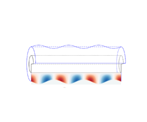
We consider a Newtonian liquid film coating on a horizontal fibre of radius $a$ with the $x$-axis along the centreline (figure 1). The initial radius of the film measured from the $x$-axis is $r = h_0$.

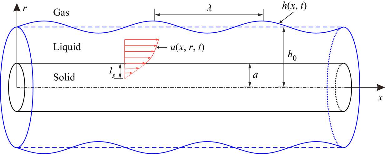
Figure 1. Schematic of a liquid film on a fibre.

The incompressible NS equations are employed to predict the dynamics of the flow inside the liquid film. To identify the governing dimensionless parameters, we non-dimensionalise the NS equations with the rescaling variables

(2.1a–d)\begin{equation} (x,r,h)= \frac{(\tilde{x},\tilde{r},\tilde{h})}{h_0}, \quad t =\frac{\gamma}{\mu h_0}\, \tilde{t}, \quad \boldsymbol{u} =\frac{\mu}{\gamma}\,\tilde{\boldsymbol{u}}, \quad (p,\boldsymbol{\tau}) = \frac{h_0}{\gamma}\,(\tilde{p},\tilde{\boldsymbol{\tau}}), \end{equation}

where $\tilde {h}$, $\tilde {t}$, $\tilde {\boldsymbol {u}}$ and $\tilde {p}$ represent the dimensional interface height, time, velocity and pressure, respectively (note that the dimensional material parameters are not given tildes). Also, $\tilde {\boldsymbol {\tau }}$ is the shear stress, which is proportional to the strain rate in Newtonian fluids, $\mu$ is the liquid dynamic viscosity, and $\gamma$ is the surface tension of the liquid–gas interface. The dimensionless NS equations can be written as

(2.2)$$\begin{gather} \boldsymbol{\nabla}\boldsymbol{\cdot} \boldsymbol{u} =0 , \end{gather}$$

(2.3)$$\begin{gather}\partial_{t} \boldsymbol{u}+ \boldsymbol{u} \boldsymbol{\cdot} \boldsymbol{\nabla} \boldsymbol{u} = {Oh}^2\,( \boldsymbol{\nabla} \boldsymbol{\cdot}\boldsymbol{\tau} - \boldsymbol{\nabla} p ) . \end{gather}$$

The non-dimensional quantity ${Oh}=\mu /\sqrt {\rho \gamma h_0}$ is the Ohnesorge number, which relates the viscous forces to inertial and surface-tension forces. Note that in the previous experiment for the slip-enhanced RP instability (Haefner et al. 2015), a high-viscosity polymer liquid, entangled polystyrene, is coated on a fibre with radius $10\unicode{x2013}25\ \mathrm {\mu }\mathrm {m}$. The density of the entangled polystyrene is $\rho =1.05\ \mathrm {g}\ \mathrm {cm}^{-3}$, and its liquid–gas surface tension is $\gamma = 30.8\ \mathrm {mN}\ \mathrm {m}^{-1}$. The liquid viscosity depends on temperature, with various values in the range $0.2\unicode{x2013}10\ \mathrm{kg}\ \mathrm {m}^{-1}\ \mathrm {s}^{-1}$ (Haefner 2015). So the Ohnesorge number of liquid film in the experiment is larger than 10, and ${Oh}^2 \gg 1$ in (2.3). It is reasonable to assume that the inertial terms are negligible compared to the viscous terms. With axisymmetric initial perturbations, (2.2) and (2.3) can be reduced to axisymmetric Stokes equations, written as

(2.4)$$\begin{gather} \frac{\partial u}{\partial x} + \frac{1}{r}\,\frac{\partial (vr)}{\partial r} = 0 , \end{gather}$$

(2.5)$$\begin{gather}\frac{\partial p}{\partial x} = \frac{\partial^2 u}{\partial x^2} + \frac{1}{r}\,\frac{\partial}{\partial r} \left( r\,\frac{\partial u}{\partial r} \right) , \end{gather}$$

(2.6)$$\begin{gather}\frac{\partial p}{\partial r} = \frac{\partial^2 v}{\partial x^2} + \frac{\partial}{\partial r} \left[\frac{1}{r}\,\frac{\partial (vr)}{\partial r}\right], \end{gather}$$

where $u$ and $v$ represent the axial and radial velocities, respectively. Since the density of gas around the film is much smaller than that of liquid, the gas flow outside can be assumed to be dynamically passive to simplify the problem. The liquid–gas interface height $h(x,t)$ satisfies the kinematic boundary condition

(2.7)\begin{equation} \frac{\partial h}{\partial t} + u\,\frac{\partial h}{\partial x} = v. \end{equation}

The normal stress balances at the interface $r=h$ give

(2.8)\begin{equation} p- \boldsymbol{n} \boldsymbol{\cdot} \boldsymbol{\tau} \boldsymbol{\cdot} \boldsymbol{n} = \boldsymbol{\nabla}\boldsymbol{\cdot} \boldsymbol{n} , \end{equation}

where $\boldsymbol {n}$ is the outward normal, and $\boldsymbol {\nabla } \boldsymbol {\cdot } \boldsymbol {n}$ represents the dimensionless Laplace pressure. The tangential force balance is

(2.9)\begin{equation} \boldsymbol{n} \boldsymbol{\cdot} \boldsymbol{\tau} \boldsymbol{\cdot} \boldsymbol{t}=0 , \end{equation}

where $\boldsymbol {t}$ is the tangential vector. With $\boldsymbol {n}$ and $\boldsymbol {t}$ expressed in terms of the unit vectors in the $x$-direction ($\hat {\boldsymbol {e}}_x$) and $r$-direction ($\hat {\boldsymbol {e}}_r$), i.e.

(2.10a,b)\begin{align} \boldsymbol{n} ={-}\frac{\partial_x h}{\sqrt{1+(\partial_x h)^2}}\,\hat{\boldsymbol{e}}_x + \frac{1}{\sqrt{1+(\partial_x h)^2}}\,\hat{\boldsymbol{e}}_r \quad\textrm{and}\quad \boldsymbol{t} = \frac{1}{\sqrt{1+(\partial_x h)^2}}\,\hat{\boldsymbol{e}}_x + \frac{\partial_x h}{\sqrt{1+(\partial_x h)^2}}\,\hat{\boldsymbol{e}}_r, \end{align}

(2.8) and (2.9) give explicitly

(2.11)\begin{align} &p - \frac{2}{1+ \left(\partial_x h \right)^2} \left[ \frac{\partial v}{\partial r} - \frac{\partial h}{\partial x} \left( \frac{\partial u}{\partial r} + \frac{\partial v}{\partial x}\right) + \left(\frac{\partial h}{\partial x} \right)^2 \frac{\partial u}{\partial x} \right] \nonumber\\ &\quad =\frac{1}{h \sqrt{1+\left(\partial_x h \right)^2}} - \frac{\partial_x^2 h}{\left(1+\left(\partial_x h \right)^2\right) ^{3/2}} \end{align}

for the normal forces, and

(2.12)\begin{equation} 2\,\frac{\partial h}{\partial x} \left( \frac{\partial v}{\partial r} - \frac{\partial u}{\partial x} \right) + \left[ 1- \left(\frac{\partial h}{\partial x} \right)^2 \right] \left( \frac{\partial u}{\partial r} + \frac{\partial v}{\partial x} \right) = 0 \end{equation}

for the tangential forces. Here, $\partial _x$ and $\partial _x^2$ refer to first and second spatial derivatives. In terms of the boundary conditions at the fibre surface $r = \alpha$ (where $\alpha$ is the dimensionless fibre radius, i.e. $\alpha = a/h_0$), we have the slip boundary condition in the tangential direction and the no-penetration boundary condition in the normal direction, such that

(2.13a,b)\begin{equation} u = l_{s}\,\frac{\partial u}{\partial r}, \quad v=0. \end{equation}

Here, $l_{s}$ represents the dimensionless slip length rescaled by $h_0$. The governing equations above can be simplified further under the long-wave approximation to give a one-dimensional lubrication equation, compared with experimental results in the previous work (Haefner et al. 2015). This lubrication equation is displayed here for the instability analysis appearing in § 3 (see Appendix A for the derivation). Its dimensionless format is

(2.14)\begin{equation} \frac{\partial h}{\partial t} = \frac{1}{ h}\,\frac{\partial}{\partial x} \left[ M(h)\, \frac{\partial p}{\partial x} \right], \end{equation}

where $M(h)$ is the mobility term

(2.15)\begin{equation} M(h) =\frac{1}{16} \left[{-}3h^4-\alpha^4 + 4 \alpha^2 h^2 + 4 h^4 \ln\left(\frac{h}{\alpha}\right) + 4 l_{s}\,\frac{(h^2-\alpha^2)^2}{\alpha} \right], \end{equation}

and $p$ is the Laplace pressure

(2.16)\begin{equation} p = \frac{1}{h} - \frac{\partial^2 h}{\partial x^2} . \end{equation}

3. Instability analysis

In this section, linear instability analysis based on (2.4)–(2.13a,b) is performed using the normal mode method, which has been used widely for the RP instability in different fluid configurations (Rayleigh 1878; Tomotika 1935; Craster & Matar 2006; Liang et al. 2011). The dimensionless perturbed quantities are expressed as

(3.1)\begin{equation} \left.\begin{gathered} u(x,r,t) = \hat{u}(r) \exp({\omega t+{\rm i}kx}),\quad v(x,r,t) = \hat{v}(r) \exp({\omega t+{\rm i}kx})\\ \textrm{and}\quad p(x,r,t) = 1 + \hat{p}(r) \exp({\omega t+{\rm i}kx}), \end{gathered}\right\} \end{equation}

where $\omega$ is the growth rate of perturbations, and $k$ is the wavenumber. Substituting these quantities into the mass and momentum equations (2.4)–(2.6) leads to

(3.2)$$\begin{gather} {\rm i}k \hat{u} + \frac{1}{r}\,\frac{{\rm d} (\hat{v} r)}{{\rm d} r} = 0 , \end{gather}$$

(3.3)$$\begin{gather}{\rm i}k \hat{p} ={-}k^2 \hat{u} + \frac{1}{r}\,\frac{{\rm d}}{{\rm d} r} \left( r\,\frac{ {\rm d} \hat{u}}{{\rm d} r} \right) , \end{gather}$$

(3.4)$$\begin{gather}\frac{{\rm d} \hat{p}}{{\rm d} r} ={-}k^2 \hat{v} + \frac{{\rm d}}{{\rm d} r}\left[\frac{1}{r}\,\frac{{\rm d} (\hat{v} r)}{{\rm d} r}\right] . \end{gather}$$

With (3.2)–(3.4), we can eliminate $\hat {u}$ and $\hat {p}$ to get a fourth-order ordinary partial differential equation for $\hat {v}$:

(3.5)\begin{equation} \frac{{\rm d} }{{\rm d} r}\left\lbrace\frac{1}{r}\,\frac{{\rm d}}{{\rm d} r} \left[r\,\frac{{\rm d}}{{\rm d} r} \left(\frac{1}{r}\,\frac{{\rm d}(\hat{v}r)}{{\rm d}r} \right) \right] \right\rbrace - 2k^2\, \frac{{\rm d}}{{\rm d}r}\left[\frac{1}{r}\,\frac{{\rm d}(\hat{v}r)}{{\rm d}r} \right]+k^4\hat{v} = 0 . \end{equation}

The general solution for (3.5) can be obtained in terms of Bessel functions, written as

(3.6)\begin{equation} \hat{v} = C_1 r\,{\rm K}_0(kr) + C_2\,{\rm K}_1(kr)+ C_3 r\,{\rm I}_0(kr) + C_4\, {\rm I}_1(kr) , \end{equation}

where I and K are modified Bessel function of the first and second kinds, the subscripts $0$ and $1$ represent the order of the Bessel functions, $C_1\unicode{x2013} C_4$ are four arbitrary constants to be determined by the boundary conditions, and $r\in [\alpha,1]$. Substituting (3.6) into (3.2) and (3.3) gives us the solutions for $\hat {u}$ and $\hat {p}$:

(3.7)$$\begin{gather} \hat{u} = \left[ C_1 ( kr\,{\rm K}_1-2\,{\rm K}_0 )+ C_2 k\,{\rm K}_0 - C_3(2\,{\rm I}_0 + kr\,{\rm I}_1 ) - C_4 k\,{\rm I}_0 \right] / ({\rm i}k) , \end{gather}$$

(3.8)$$\begin{gather}\hat{p} = 2 ( C_1\,{\rm K}_0 + C_3\,{\rm I}_0 ) . \end{gather}$$

In a similar approach, the dimensionless perturbed quantities for $\hat {u}, \hat {v}, \hat {p}$, combined with $h(x,t) = 1 + \hat {h}\exp ({\omega t+\textrm {i}kx})$, are substituted into perturbed boundary equations (2.7)–(2.13a,b). For the boundary conditions at the interface ($r=1$), their linearisation gives

(3.9)$$\begin{gather} \frac{{\rm d} \hat{u}}{{\rm d} r} + {\rm i}k \hat{v} = 0, \end{gather}$$

(3.10)$$\begin{gather}\hat{p} - 2\,\frac{{\rm d} \hat{v}}{{\rm d} r} = \hat{h} (k^2-1 ), \end{gather}$$

(3.11)$$\begin{gather}\omega \hat{h} = \hat{v} . \end{gather}$$

And for the boundary conditions on the fibre surface ($r=\alpha$), their linearised forms are

(3.12)$$\begin{gather} \hat{u} = l_{s}\,\frac{{\rm d} \hat{u}}{{\rm d} r}, \end{gather}$$

(3.13)$$\begin{gather}\hat{v} = 0 . \end{gather}$$

According to (3.11), $\hat {h}$ in (3.10) can be eliminated to give the final four equations of the boundary conditions, i.e. (3.9), (3.10), (3.12) and (3.13). Substituting the Bessel functions (3.6)–(3.8) into these perturbed equations leads to a homogeneous system of linear equations for $C_1\unicode{x2013} C_4$, which has a non-trivial solution only if the determinant of the coefficients vanishes. In this way, we have the final equation

(3.14)\begin{equation} \left|\begin{array}{@{}cccc@{}} F_{11} & F_{12} & F_{13} & F_{14} \\ F_{21} & F_{22} & F_{23} & F_{24} \\ \alpha\,{\rm K}_0(k \alpha) & {\rm K}_1(k \alpha) & \alpha\,{\rm I}_0(k \alpha) & {\rm I}_1(k \alpha) \\ k\,{\rm K}_0(k) - {\rm K}_1(k) & k\,{\rm K}_1(k) & k\,{\rm I}_0(k) + {\rm I}_1(k) & k\,{\rm I}_1(k) \\ \end{array}\right| =0 , \end{equation}

where

(3.15)\begin{equation} \left.\begin{gathered} F_{11} = (k^2-1)\,{\rm K}_0(k) - 2 \omega k\,{\rm K}_1(k), \\ F_{12} = (k^2-1)\,{\rm K}_1(k) - 2 \omega \left[ k\,{\rm K}_0(k) + {\rm K}_1(k) \right], \\ F_{13} = (k^2-1)\,{\rm I}_0(k) + 2 \omega k\,{\rm I}_1(k) , \\ F_{14} = (k^2-1)\,{\rm I}_1(k) + 2 \omega \left[ k\,{\rm I}_0(k) - {\rm I}_1(k) \right], \\ F_{21} = (2-l_{s} k^2 \alpha)\,{\rm K}_0(k \alpha) + k(2 l_{s}-\alpha)\,{\rm K}_1(k \alpha) , \\ F_{22} ={-}k\,{\rm K}_0(k \alpha) - l_{s} k^2\,{\rm K}_1(k \alpha), \\ F_{23} = (2-l_{s} k^2 \alpha)\,{\rm I}_0(k \alpha) -k(2 l_{s}-\alpha)\,{\rm I}_1(k \alpha) , \\ F_{24} = k\,{\rm I}_0(k \alpha) - l_{s} k^2\,{\rm I}_1(k \alpha). \end{gathered}\right\} \end{equation}

Because $\omega$ appears only linearly in the first line of the determinant, the dispersion relation between $\omega$ and $k$ can be expressed explicitly as

(3.16)\begin{align} \omega = \frac{k^2-1}{2}\,\frac{{\rm K}_0(k)\,\varDelta_1 - {\rm K}_1(k)\,\varDelta_2 + {\rm I}_0(k)\,\varDelta_3 -{\rm I}_1(k)\,\varDelta_4}{k\,{\rm K}_1(k)\,\varDelta_1- \left[ k\,{\rm K}_0(k)+{\rm K}_1(k) \right] \varDelta_2 -k\,{\rm I}_1(k)\,\varDelta_3 + \left[ k\,{\rm I}_0(k) -{\rm I}_1(k) \right] \varDelta_4} , \end{align}

where

(3.17)\begin{equation} \left.\begin{gathered} \varDelta_1 = \left|\begin{array}{@{}ccc@{}} F_{22} & F_{23} & F_{24} \\ {\rm K}_1(k \alpha) & \alpha\,{\rm I}_0(k \alpha) & {\rm I}_1(k \alpha) \\ k\,{\rm K}_1(k) & k\,{\rm I}_0(k) + {\rm I}_1(k) & k\,{\rm I}_1(k) \end{array}\right|, \\ \varDelta_2 = \left|\begin{array}{@{}ccc@{}} F_{21} & F_{23} & F_{24} \\ \alpha\,{\rm K}_0(k \alpha) & \alpha\,{\rm I}_0(k \alpha) & {\rm I}_1(k \alpha) \\ k\,{\rm K}_0(k) - {\rm K}_1(k) & k\, {\rm I}_0(k) + {\rm I}_1(k) & k\,{\rm I}_1(k) \end{array}\right|, \\ \varDelta_3 = \left|\begin{array}{@{}ccc@{}} F_{21} & F_{22} & F_{24} \\ \alpha\,{\rm K}_0(k \alpha) & {\rm K}_1(k \alpha) & {\rm I}_1(k \alpha) \\ k\,{\rm K}_0(k) - {\rm K}_1(k) & k\,{\rm K}_1(k) & k\,{\rm I}_1(k) \end{array}\right|, \\ \varDelta_4 = \left|\begin{array}{@{}ccc@{}} F_{21} & F_{22} & F_{23} \\ \alpha\,{\rm K}_0(k \alpha) & {\rm K}_1(k \alpha) & \alpha\,{\rm I}_0(k \alpha) \\ k\,{\rm K}_0(k) - {\rm K}_1(k) & k\, {\rm K}_1(k) & k\,{\rm I}_0(k) + {\rm I}_1(k) \end{array}\right|. \end{gathered}\right\} \end{equation}

To compare the Stokes model (3.16) with the lubrication theory, (2.14) is linearised using $h = 1 + \hat {h} \exp ({\omega t + \textrm {i}kx})$, providing the dispersion relation

(3.18)\begin{equation} \omega = (k^2-1) k^2 M, \end{equation}

where $M =[3+ \alpha ^4 - 4 \alpha ^2 + 4 \ln \alpha - 4 l_{s} (1-\alpha ^2)^2/\alpha ]/16.$

In figure 2, predictions of (3.16) and (3.18) in the limiting case ($l_{s}=0$) are found to agree with the results of Craster & Matar (2006). Note that the lubrication dispersion relation (dashed lines) matches the Stokes dispersion relation (solid lines) when $\alpha \geqslant 0.6$. However, the agreement deteriorates for the smaller $\alpha$, mainly due to the limitations of lubrication approximations for ‘thicker’ films. Despite the failure in predicting the dispersion relation for small $\alpha$, the Plateau instability criterion with critical wavenumber, $k_{crit}=2{\rm \pi} h_0/\lambda _{crit}=1$ (Plateau 1873), can be predicted by the lubrication model for all $\alpha$ values. The reason is that both the circumferential and tangential curvature for the Laplace pressure are kept in (2.16) to give the term $k^2-1$ in the dispersion relation.

Figure 2. The dispersion relation between the growth rate $\omega$ and the wavenumber $k$ on the no-slip boundary condition ($l_{s}=0$) for various dimensionless fibre radii: (a) $\alpha =0.7$ (black), $\alpha =0.6$ (red), $\alpha =0.5$ (blue); (b) $\alpha =0.3$ (black), $\alpha =0.2$ (red), $\alpha =0.1$ (blue). The predictions of the Stokes model (3.16) are plotted in solid lines, and results from the lubrication model (3.18) are illustrated in dashed lines. The triangles and circles are the long-wave and Stokes results of Craster & Matar (2006), employed here to verify (3.16) and (3.18), respectively.

Figure 3 illustrates the dispersion relations of different $l_{s}$ values. Both the Stokes model and the lubrication model show that the RP instability is enhanced by slip with faster growing perturbations for larger $l_{s}$, consistent with previous findings based on lubrication models (Liao et al. 2013; Haefner et al. 2015; Halpern & Wei 2017). However, obvious discrepancies between the Stokes dispersion relation and the lubrication dispersion relation are found in most cases in figure 3. Even for thin films ($\alpha \geqslant 0.7$), where the lubrication model has been shown to perform well on the no-slip boundary condition (see the agreement of black lines in figures 3a,b), remarkable discrepancies appear when $l_{s} \geqslant 0.5$, indicating that the lubrication model (2.14) is not suitable for large-slip cases. The main reason is that the lubrication approximation imposes a restriction on $l_{s}$, namely $l_{s} \ll \lambda ^2 -1+\alpha$, where $\lambda$ is the perturbation wavelength (see the derivation of (A30) and its corresponding explanation in Appendix A). Moreover, the discrepancy increases for larger $\alpha$, similar to the trend found in the no-slip cases in figure 2.

Figure 3. The dispersion relation between the growth rate $\omega$ and the wavenumber $k$ on different boundary conditions of various dimensionless fibre radii: (a) $\alpha =0.9$, (b) $\alpha =0.7$, (c) $\alpha =0.5$, (d) $\alpha =0.3$. The solid and dashed lines are the predictions of the Stokes model (3.16) and the lubrication model (3.18), respectively, on three boundary conditions with $l_{s}=0$ (black), $l_{s}=0.25$ (blue) and $l_{s}=0.5$ (red).

The $k_{crit}$ values for the RP instability in figure 3 are found to be not affected by the slip. These values are determined by the competition between the two curvature terms for the Laplace pressure, shown on the right-hand side of (2.11), where the term of the circumferential curvature $1/ (h \sqrt {1+(\partial _x h )^2} )$ is the driving force, and the term of tangential curvature $\partial _x^2 h/ (1+(\partial _x h )^2) ^{3/2}$ is the resisting force. The balance of the two forces gives $k_{crit}$, which is independent of $l_{s}$. The dominant wavenumber $k_{max}$ predicted by the Stokes model in figure 3 is shown to be modified by slip, while $k_{max}$ from the lubrication model is unchanged with an analytical expression $k_{max} = \sqrt {1/2}$, derived from (3.18). The variations of $k_{max}$ with slip are illustrated further in figure 4(a), where $k_{max}$ declines with increasing $l_{s}$, possibly leading to larger drop sizes after the film breakup. This trend holds for different fibre radii with more rapid decrease of $k_{max}$ of thicker films (smaller $\alpha$). These findings indicate the limitations of the classical slip lubrication models (Liao et al. 2013; Haefner et al. 2015; Halpern & Wei 2017; Chao et al. 2018; Ji et al. 2019), which can be severe with large slip, while the Stokes model proposed here has the capability of predicting the instability over a much larger range of $l_{s}$. Additionally, the lubrication model shows that corresponding growth rates $\omega _{max}$ of each $k_{max}$ grow linearly with increasing $l_{s}$, which can be described by $\omega _{max} = -M/4$, while the Stokes model presents nonlinear growth with smaller $\omega _{max}$.

Figure 4. Variations of the dominant wavenumber $k_{max}$ and corresponding growth rate $\omega _{max}$ with slip lengths. The solid and dashed lines are the predictions of the Stokes model (3.16) and the lubrication model (3.18), respectively, for different fibre thicknesses, i.e. $\alpha =0.9$ (black), $\alpha =0.7$ (blue), $\alpha =0.5$ (red) and $\alpha =0.3$ (purple).

4. Numerical simulations

In this section, direct numerical simulations are performed to support the theoretical findings in § 3 and provide more physical insights into the slip-enhanced RP instability of the cylindrical films on fibres. The open-source framework Basilisk (Popinet 2014, 2018) is employed to solve axisymmetric incompressible NS equations with surface tension. The interface between the high-density liquid and the low-density ambient air is reconstructed by a volume-of-fluid method, which has been validated by different kinds of interfacial flows such as jet breakup (Deblais et al. 2018), bubble bursting (Berny et al. 2020) and breaking waves (Mostert & Deike 2020).

The simulation domain is a rectangle (the section of a hollow cylinder in cylindrical coordinates) of size $[\alpha, 2]\times [0, L]$. Here, $L$ is the length of the film/fibre, and $\alpha$ is the radius of the fibre. The liquid film of initial radius $h_0 = 1$ is placed at the bottom of the domain, with small perturbations at the liquid–gas interface. The left and right boundary conditions of the simulation domain are considered periodic. The top is a symmetry boundary and bottom is a slip-wall boundary, as described by (2.13a,b). All simulations are performed in the dimensionless unit with the rescaling variables displayed in (2.1a–d). The non-dimensional parameter ${Oh}=10$ comes from liquid properties displayed in the previous experiment (Haefner 2015) with $h_0 = 10\ \mathrm {\mu }\mathrm {m}$, $\rho =1.05\ \mathrm {g}\ \mathrm {cm}^{-3}$, $\gamma = 30.8\ \mathrm {mN}\ \mathrm {m}^{{-1}}$ and $\mu =0.22\ \mathrm {kg}\ \mathrm {m}^{-1}\ \textrm {s}^{{-1}}$. Two configurations with different film lengths and initial perturbations are simulated here to investigate the influence of slip on the growth rates of perturbations (§ 4.1) and the dominant wavelength (§ 4.2), respectively.

4.1. Influence of slip on perturbation growth rates

To study the influence of slip on the growth rates, we consider simulations of a relatively short film $L=10$ with an initial perturbation $h(x,t) =1+ \varepsilon \cos [2 {\rm \pi}(x/L-1/2)]$, where $\varepsilon =0.01$. High-density grids are employed to capture the interface position and velocity profiles inside the film, with $2^{10}$ grid points along the $x$-axis. We choose three slip lengths, i.e. $l_{s}=0$, $0.25$ and $0.5$, for two fibre radii, $\alpha =0.7$ and $0.5$.

Figure 5 shows the simulation results on a no-slip fibre of the radius $\alpha =0.7$. The upper half of figure 5 shows a time evolution of the interface positions of the film, with the initial perturbations starting to grow due to the RP instability. The axial velocity $u(x,r)$ is crucial to understand influence of the slip on the fibre thinning, shown in the lower half of figure 5, where opposite fluxes are found to be directed towards the left and right boundaries, respectively, as the perturbation increases. More velocity fields are presented in figures 6(a,c,e) for three different slip lengths at $t=100$. According to the variations of the contours in figures 6(a,c,e), the wall slip is found to accelerate the instability with larger $u(x,r)$. The velocity vectors in the lower plots of figures 6(a,c,e) show that slip decreases the velocity gradient $\partial u/ \partial r$ near the fibre. The velocity profiles at different $x$-coordinates (see the dashed lines with arrows in figures 6a,c,e) are also extracted from the contours, shown in figures 6(b,d, f), where the velocity on the fibre $u(x,\alpha )$ and its gradient $\partial _r u(x,\alpha )$ are calculated numerically. According to (2.13a,b), $l_{s} = u(x,\alpha ) / \partial _r u(x,\alpha )$. So we can have numerically predicted slip lengths at different positions, shown by the dashed lines in figures 6(d, f). These values agree with the input $l_{s}$ in the boundary condition of the simulations, indicating that the numerical solutions can capture the flow features on the slip boundary conditions.

Figure 5. Film thinning simulation results of one perturbation wave in an axially symmetric domain. For this case, $L=10$, $l_{s}=0$ and $\alpha =0.7$. Interface profiles $h$ (upper half) and contours of the axial velocity $u(x,r,t)$ inside the film (lower half) are shown at three time instants: (a) $t_1=300$, (b) $t_2=600$, (c) $t_3=900$. Here, $h_{min}$ represents the minimum radius of the film.

Figure 6. Axial velocity fields at $t=100$ for different slip lengths: (a,b) $l_{s} = 0$, (c,d) $l_{s} = 0.25$, (e, f) $l_{s} = 0.5$. Here, the fibre radius is $\alpha = 0.7$. (a,c,e) Contours of the entire configuration (upper plots) and velocity vectors of the local field near $x=6$ (lower plots). (b,d, f) Velocity profiles at four local positions $x$: $5.5$ (black), 6.0 (purple), 6.5 (blue) and 7.0 (red), shown by dashed lines with arrows in (a,c,e).

Figure 7 illustrates the growth rates of perturbations in the six cases simulated here. Because $h(x,t) = 1+\hat {h}\,\textrm {e}^{\textrm {i}kx}\,\textrm {e}^{\omega t}$ is employed in the instability analysis (§ 3), we set the $y$-coordinate as $\ln (1-h_{min})$ to present the linear growth of perturbations. Here, the numerical solutions agree with predictions of the Stokes model, showing the capability of the Stokes model to describe the RP instability of films on slippery fibres, while the predictions of the lubrication model are not accurate for the slip cases. These results are consistent with dispersion relations in figure 3 and confirm the Stokes model numerically.

Figure 7. Linear time evolution of the minimum radii of films $h_{min}(t)$ on two fibre radii: (a) $\alpha =0.7$, (b) $\alpha =0.5$. The numerical solutions (dotted lines with symbols) are compared to the predictions of both the lubrication model (dashed lines) and Stokes model (solid lines) for three slip lengths: $l_{s} = 0$ (black), $l_{s}=0.25$ (red) and $l_{s}=0.5$ (blue). The inset illustrates $h_{min}(t)$ in the uniform grids. Here, $t$ is scaled by $\mu h_0/\gamma$.

Based on the approach proposed by Liao et al. (2013) and Wei, Tsao & Chu (2019), we have a physical explanation for why large slip causes the failure of lubrication models, i.e. the radial derivative of the axial velocity is no longer much larger than its axial derivative, violating the lubrication approximation $| {\partial ^2 u}/{\partial x^2} | / |({1}/{r}) ({\partial }/{\partial r})(r ({\partial u}/{\partial r}) )| \ll 1$ (see more details in Appendix A). Figure 8 shows the contour inside the film of the ratio $| {\partial ^2 u}/{\partial x^2} | / |({1}/{r})({\partial }/{\partial r})(r ({\partial u}/{\partial r}) )|$, extracted from the numerical solutions in this section. The ratio is found to increase from about $0.01$ for the no-slip case to $0.1$ for the slip case ($l_{s}=0.5$) at the same location, which is consistent with the physical explanation above.

Figure 8. Ratio of the velocity gradients at $t=100$ for different slip lengths: (a) $l_{s} = 0$, (b) $l_{s} = 0.25$, (c) $l_{s} = 0.5$. Here, the fibre radius is $\alpha = 0.7$, and $u_{xx}$ and $(r u_r)_r/r$ represents the second-order axial and radial derivatives of the axial velocity in (A24), respectively.

4.2. Influence of slip on the dominant wavelength

For the influence of slip on the dominant wavelengths, we consider a configuration of a long film $L=160$ with $2^{13}$ grid points along the $x$-axis. Eight different cases are simulated with four slip lengths, i.e. $l_{s}=0$, $1$, $2$ and $3$ on fibres of two radii, $\alpha =0.7$ and $0.5$.

The simulations start from random initial perturbations $h(x,0) = 1+ \varepsilon \,N(x)$, where $\varepsilon = 2 \times 10^{-3}$, and the random number $N(x)$ follows a normal distribution with zero mean and unit variance. The random initial perturbations are designed to mimic numerically the arbitrary disturbances in the experiment (Haefner et al. 2015). Figure 9 presents the spatial and temporal evolutions of interface profiles $h(x,t)$, where these small random perturbations, driven by the surface tension in the RP instability, grow gradually against time to generate significant capillary waves at early stages, plotted in figure 9(b). Figure 9(c) shows that wavelengths of these capillary waves are unchanged at the later stage of perturbation growth.

Figure 9. (a) Space–time plot of interface positions $h(x,t)$ on a no-slip fibre of the radius $\alpha =0.7$. Darker (brighter) colours correspond to the smaller (larger) values of $h(x,t)$. (b,c) Interface profiles extracted from (a) at early and late stages of the instability.

To further prove the previous findings and confirm theoretical predictions of the Stokes model quantitatively, multiple independent simulations (five for each case) are performed to gather statistics of the dominant modes with a statistical methodology proposed by Zhao, Sprittles & Lockerby (2019). For each realisation, a discrete Fourier transform of the interface position $h(x)$ is applied to get the power spectral density (PSD) of the perturbations. The square root of the ensemble-averaged PSD ($H_{rms}$) at each time is plotted in figures 10(a,b) with a modal distribution (spectrum) fitted by the Gaussian function, where the peak represents the dominant wavenumber $k_{max}$ (see black dash-dotted lines). Extracting $k_{max}$ from the fitted spectrum at each time instant yields the insets in figures 10(a,b). Promisingly, $k_{max}$ converges rapidly to a constant in both cases, further supporting the findings in figure 9(c). Here, we compare these constants with the $k_{max}$ predicted by the Stokes model. Similar statistical analysis is applied for other cases to generate the symbols ($\lambda _{max} = 2 {\rm \pi}/k_{max}$) in figure 10(c), giving good agreement with theoretical predictions. Therefore, we can conclude that the dominant modes depend strongly on slip lengths with longer perturbation waves formed on a more slippery surface.

Figure 10. (a,b) The root mean square (r.m.s.) of non-dimensional perturbation amplitude versus non-dimensional wavenumber on fibres with different slip lengths, at four time instants: (a) $2\times 10^3$ (green), $4.5\times 10^3$ (black), $6\times 10^3$ (red) and $7\times 10^3$ (blue); (b) $1.2\times 10^2$ (green), $3.3\times 10^2$ (black), $4.2\times 10^2$ (red) and $4.8\times 10^2$ (blue). The inset shows the time history of the dominant wavenumber. (c) Variations of the dominant wavelengths with slip lengths: a comparison between the theoretical predictions of (3.16) and numerical solutions for two fibres of different radii.

Figure 11 shows the influence of slip on the droplet size. In figure 11(a), larger drops are formed on slippery fibres with obviously longer wavelengths compared to ones achieved on the no-slip boundary, consistent with the theoretical results in figure 10(c) qualitatively. Furthermore, we define the area between two bottom points of $h(x)$ as one droplet. Performing statistical analysis for all realisations gives the droplet-size distribution of slip and no-slip cases, illustrated in figure 11(b), whose mean and standard deviation are achieved by fitting the Gaussian function (red dash-dotted lines). The slip case has a larger mean value of the distribution, further proving the finding in figure 11(a). Besides the mean, slip is also found to lead to a wider distribution, with a larger standard deviation, possibly because the slip wall imposes fewer restrictions (shear stresses on the fibre, i.e. $\tilde {\tau }_{w} = \mu \,\partial _{\tilde {r}} \tilde {u}(\tilde {x},a)$) on the liquid compared to the no-slip wall. The perturbation wavelengths have more ‘freedom’ to expand or shrink, leading to a wider wavelength distribution. Note that figure 11 might not be the final equilibrium state. So droplet coalescence could happen with complicated nonlinear dynamics. However, these nonlinear behaviours are beyond the scope of this work and should be the subject of future investigation.

Figure 11. (a) Interface profiles of liquid films on fibres of radius $\alpha =0.7$. The results for two slip lengths are presented by a solid blue line for $l_{s}=0$, and a red dash-dotted line for $l_{s}=3$. (b) Distributions of the droplet size on the no-slip (upper plot) and slip (lower plot).

5. Comparisons with experimental results

Besides the numerical validations, the Stokes model is compared further with the experimental results in the previous work done by Haefner et al. (2015). The experiments were done by measuring the evolutions of entangled polystyrene films with homogeneous initial thicknesses on no-slip and slip fibres of radius $a=9.6\ \mathrm {\mu }\textrm {m}$.

Figure 12 displays the dimensional dominant wavelengths $\tilde {\lambda }_{max}$ ($\lambda _{max} h_0$) of liquid films with different initial thicknesses $h_0$, where the blue triangles and red dots represent experimental data of the films on no-slip and slip fibres, respectively. Since $\lambda _{max}$ predicted by the lubrication model (3.18) is the constant ($\lambda _{max}=2\sqrt {2}{\rm \pi}$), independent of both $l_{s}$ and $\alpha$, $\lambda _{max} h_0$ grows linearly with increasing $h_0$ (see the black dashed line in figure 12). However, the lubrication model seemingly underestimates experimentally obtained $\lambda _{max}$. The possible reason is that most $\alpha$ values investigated in the experiment are smaller than $0.5$, outside the range of validity of the lubrication approximation. A series of dominant wavelengths with different $\alpha$ values are extracted from the Stokes model (3.16) to generate a blue solid line for no-slip cases, and a red dash-dotted line for slip cases with a fitting $\tilde {l}_{s}$ in figure 12. Note that the dimensionless slip length varies along the red dash-dotted curve with different $h_0$ values. Though both the blue and red curves still look linear due to small changes of $\lambda _{max}$, obvious differences between the Stokes predictions and the lubrication ones are found for the thick films ($h_0>40\ \mathrm {\mu }\textrm {m}$). Promisingly, despite dispersion of experimental data, the Stokes model can provide better predictions for dominant wavelengths of both no-slip cases and slip cases compared to the lubrication model.

Figure 12. Influence of the geometry on the dominant wavelength of the instability: a comparison between the theoretical predictions and experimental data. The experimental data come from the work of Haefner et al. (2015).

In addition to the dominant wavelengths, we then make a further comparison between the experimental growth rates and theoretical ones, illustrated in figure 13, where the growth rate is non-dimensionalised by the ratio of the capillary velocity to the fibre radius, i.e. $\omega =({a}\tilde {\omega }/({\gamma /\mu }))$. However, using the parameters from Haefner et al. (2015) ($\gamma /\mu = 294\ \mathrm {\mu }\mathrm {m}\ \min ^{-1}$ and $\tilde {l}_{s} = 0.3\,a$), the Stokes model is found to provide worse agreements with the experimental data than the lubrication model. Noticeably, predictions of the lubrication model match the experimental data even in the case of thick films ($h_0/a > 3$), which is unreasonable due to the thin-film assumption in the lubrication theory. The reason for the disagreement is currently unclear and should be the subject of future investigation.

Figure 13. Influence of the geometry on the growth rate of the dominant mode on no-slip and slip fibres. The solid lines and dashed lines are the predictions of the Stokes model and the lubrication model, respectively. Blue lines represent no-slip results, and red lines are the slip ones. The experimental data come from the work of Haefner et al. (2015).

6. Conclusions

In this work, to study the influence of liquid–solid slip on the RP instability of liquid films on a fibre, a theoretical model based on the linear stability analysis of axisymmetric Stokes equations is developed, which goes beyond the classical slip lubrication model. The lubrication model is found to overestimate the slip-enhanced growth rates of perturbations and fails to predict the dominant wavelength, while the new model can provide more accurate predictions for the instability. Direct numerical simulations of the NS equations are then performed to validate the two theoretical findings via two fluid configurations: (i) a short film with a fixed wavelength for the slip-enhanced growth rate of the perturbation; and (ii) a long film with random initial perturbations for the slip-dependent dominant modes of perturbations. The dominant wavelengths are also confirmed by experimental data from previous work (Haefner et al. 2015). Overall, the applicability of the slip lubrication model should be restricted to thin-film and small-slip flows. For more general problems, it is better to use the Stokes theory proposed here.

Promisingly, the wall slip has been realised experimentally for films on a fibre (Haefner et al. 2015; Ji et al. 2019), and the slip length can also be measured directly (Huang, Guasto & Breuer 2006; Maali & Bhushan 2012; Maali, Colin & Bhushan 2016). It is our hope that the wall slip can be controlled experimentally to verify our new predictions, most notably the relation between drop sizes ($\lambda _{max}$) and slip lengths. Potential extensions of the framework are numerous: for example, to include the influence of other physics, such as electric fields (Ding et al. 2014) and intermolecular forces (Ji et al. 2019; Tomo et al. 2022), both of which are known to affect $k_{crit}$ and $k_{max}$ in the RP instability, and to explore related flow configurations, like a film flowing down a fibre (Liu & Ding 2021), where an interesting open problem is to understand the influence of slip on dynamics of travelling waves in different flow regimes.