Impulsive acceleration of a circular cylinder under free surface

Abstract

A present paper generalizes the work of Tyvand & Miloh (J. Fluid Mech., vol. 286, 1995, pp. 67–101) on the problem of the free surface flow generated by a submerged circular cylinder moving impulsively with constant velocity to the case of a cylinder moving with both initial velocity and acceleration. The nonlinear small-time asymptotic solution for the velocity potential, free surface elevation and hydrodynamic pressure force is calculated analytically in bipolar coordinates for a cylinder of arbitrary radius. The analytical solution is obtained to the leading order of nonlinear interaction between initial impulsive velocity and initial impulsive acceleration directed at arbitrary angles. In the special case of the motion with constant acceleration, the complete fourth-order free-surface flow problem is solved and the associated second-order hydrodynamic force is computed. The leading-order contributions to the free surface elevation due to the constant velocity and constant acceleration are compared for finite rectilinear cylinder displacements. The role of constant acceleration consists of two contributions to the leading nonlinear terms, where the amplitude of the first one is 25 % below the case of constant velocity while the amplitude of the other exceeds it by 50 %.

1. Introduction

The flow of the fluid around a submerged body moving below the free surface is a classical topic in hydrodynamics. Various aspects of this problem have been studied theoretically and in experiments by numerous investigators. Studying the disturbances created on the free surface by the motion of a submerged obstacle is relevant for prediction of wave effects on submarines, underwater pipes and submerged parts of wave-absorbing power plants. Of considerable practical importance are the unsteady hydrodynamic forces acting on a moving body in the fluid and the resulting free surface deformations. A striking application of this problem has been recently found in a field unrelated to marine hydrodynamics, namely in the magnetized target fusion power plants. Pardo et al. (2022) idealized the situation when the magnetized plasma is injected into the rotating liquid metal inside the fusion machine and then moves to the cavity in the rotating core to that of a submerged cylinder in the fluid approaching the free surface.

A cylinder of circular cross-section is generally used as a test case to avoid the difficulties of dealing with more complicated body shapes while keeping the key features of the free surface flow. For these reasons, cylinders of non-circular form have been investigated much less frequently. Kostikov & Makarenko (2016) applied a conformal mapping technique to investigate the translatory and rotary motion of an elliptic cylinder under the free surface. Semenov, Savchenko & Savchenko (2021) obtained the first-order solution for the cylinder of arbitrary cross-section moving impulsively under the undisturbed free surface by the integral hodograph method, in which the fluid region in the physical plane was mapped into the first-quadrant in the parameter plane.

Theoretical studies on the water wave problem in the presence of a submerged body can be classified into four categories, depending on whether the linear or nonlinear solution is obtained, and steady-state or transient type of motion is described.

Steady-state processes from the standpoint of linear theory are most amenable to theoretical treatment. The linearization of the free surface boundary conditions allows us to find the analytical solution to the governing equations for the fluid flow in the frequency domain at the expense of the limitation to small periodic disturbances on the free surface. Havelock (1936), after Lamb (1913), approximated the cylinder in the forced motion with constant speed under the free surface by a moving dipole in the complex plane and obtained the complete linear solution for the free surface flow. Wehausen & Laitone (1960), Dean (1948) and Ursell (1950) were particularly concerned with the linearized diffraction and radiation of water waves interacting with a circular cylinder. In these theories assuming oscillatory time dependence of the solution, the initial stage of the flow was disregarded, since all the transients are transported away from the oscillating body, when the fluid domain extends to infinity.

Ogilvie (1963) and Tuck (1965) considered the steady-state problem in the frequency domain and took weakly nonlinear effects into account. Ogilvie (1963) calculated second-order steady force in the situation when the cylinder is forced to oscillate in otherwise calm water. Tuck (1965) improved the recursive scheme developed by Wehausen & Laitone (1960) for the linear problem and built up the nonlinear solution for sufficiently deep submergence depth of the cylinder by solving a sequence of linear problems. The solution was based on the amplitude power expansion and described the stationary wave train past a horizontally moving body.

Sretensky (1937) investigated the transient problem in the linear approximation and presented the explicit analytical solution for a submerged contour of arbitrary form moving with a variable horizontal speed under the free surface. His expressions for surface elevation and fluid resistance force included integrals which were difficult to evaluate at that time. Havelock (1949), in a particular problem of a circular cylinder, starting to move impulsively from a state of rest and moving with constant velocity afterwards, demonstrated the equivalence of his solution to that of Sretensky (1937).

The transient processes in nonlinear fluid–structure interaction problems are particularly difficult to describe theoretically and hence the researchers often resort to numerical or semianalytical methods. However, some attempts to approach the problem using the perturbation techniques were made. Tyvand & Miloh (1995) found out that the problem of the cylinder starting to move impulsively from a state of rest under the free surface can be solved analytically by looking for a solution in the form of the power series. They investigated the short-time evolution of the solution with the use of small-time expansions, bipolar coordinates and Fourier series. A carefully developed temporal expansion included an infinite acceleration of the cylinder during an infinitesimal time interval. Thereby, the cylinder was instantaneously put into motion with constant velocity. By Newton's third law of motion, the associated finite momentum representing a forced fluid motion in the opposite direction occurs.

Independently, Makarenko (2003) constructed the small-time asymptotic solution for the cylinder of small radius and arrived at the same expressions for the free surface elevation. He used the method of Ovsyannikov, Makarenko & Nalimov (1985) to transform the basic equations governing the fluid flow around the moving submerged body into the boundary integro-differential system for the unknown functions on the free surface only. Later, Kostikov & Makarenko (2018) generalized this solution and described the nonlinear effects occurring in the flow around the cylinder of greater radius by taking into consideration the higher-order terms in the boundary integro-differential system. Pardo & Nedic (2021) took a further step in the development of this model and extended the small-time asymptotic solution of Kostikov & Makarenko (2018) to the higher orders with respect to time and cylinder radius by the advanced recursive semianalytical procedure. The inability to continue the asymptotic solutions beyond an uncertain time limit indicates a deficiency in either analytical or numerical models in highly nonlinear problems. However, a homotopy analysis method exists (Liao 2004), having an advantage over common analytic approximation methods of not requiring any small parameter assumption. Application of this method can improve the convergence of a series dramatically by means of the so-called convergence-control parameter. Zhong & Liao (2018) derived an approximation by use of a homotopy analysis method for the Stokes wave in highly nonlinear case of extremely shallow water.

A series of simulations based on various computational techniques were developed to study the complex unsteady nonlinear process of wave generation by a submerged cylinder in two dimensions. Haussling & Coleman (1979) used a body-fitted coordinate system and finite difference technique to construct the numerical solution of the problem. They illustrated the transition from deep submergence of the obstacle when nonlinear free surface effects are negligible to shallow submergence when linearized analysis is no longer accurate. A series of numerical calculations based on boundary integral equations and the boundary element method has been made, see for example Telste (1987), Terent'ev (1991), Greenhow & Moyo (1997) and Moyo & Greenhow (2000). Moreira & Peregrine (2010) used a fully nonlinear unsteady boundary-integral solver to study the formation of waves by a submerged cylinder in a uniform stream with surface tension. They established that in the full nonlinear formulation the wave breaking is likely to occur for the large cylinder radius to submergence depth ratio and investigated the effects of capillarity on the steepness of the free surface disturbances.

In spite of substantial progress in computer simulations of the wave–structure interaction problems, analytical methods in the description of nonlinear two-dimensional potential flows remain relevant. An initial stage of the wave formation continues to be the problem point in numerical algorithms due to the instability forming on the free surface when the submerged body starts moving. Hence, the initial stage of the body motion under a free surface is of continuing interest for scientists and engineers. In this paper, we revisit this problem by considering a circular cylinder starting to move from a state of rest with both initial velocity and initial acceleration directed at arbitrary angles. Our tasks are to investigate the interaction of these two factors, explain the role of nonlinearity in this process and to close the gaps in the work of Tyvand & Miloh (1995). It is important to be aware of the infinite acceleration needed during an infinitesimal time interval for setting the cylinder impulsively into initial motion with finite velocity. In the present work we will allow an additional finite acceleration to be maintained after the impulsive start.

More complex phenomena such as wave breaking, exit of the cylinder from under the surface, formation of cavity or splashes, the effects of fluid viscosity and surface tension are beyond the scope of the present study. Consideration of a streamlined body moving at a sufficient distance from the free surface with relatively large Froude numbers allows us to address the problem in the framework of potential theory and incompressible fluid. Despite the popularity of this problem, available experimental data are extremely limited. One of the few experimental results was reported by Greenhow & Lin (1983) for the vertical motion of the cylinder four decades ago. More recently, Pardo et al. (2022) built an experimental facility, where the liquid was impulsively accelerated around a circular cylinder, and compared the results with analytical models of Tyvand & Miloh (1995), Kostikov & Makarenko (2018) and Pardo & Nedic (2021). They showed that analytical predictions are in good agreement with the experiments for initial times.

The rest of the paper is organized as follows. In § 2, the formulation of the problem is presented and bipolar coordinates, relevant for construction of the solution, are introduced. In § 3, the leading-order nonlinear solution for the combination of impulsive velocity and impulsive acceleration is constructed, including the case of pure impulsive acceleration of the cylinder. Section 4 scrutinizes causal connections between the finite displacement of the cylinder and early non-gravitational surface elevations for the nonlinear flow problem. In § 5, the hydrodynamic forces acting on the moving cylinder are deduced. Finally, § 6 summarizes the main conclusions of the paper.

2. Formulation of the problem

2.1. Governing equations

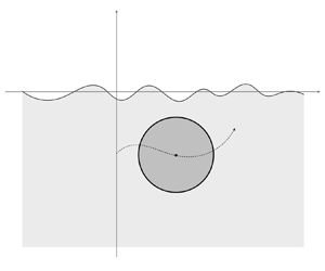
We consider the unsteady motion of a circular cylinder of radius $\varepsilon$ under the free surface of an inviscid incompressible fluid of infinite depth and constant density $\rho$. The two-dimensional flow is considered in Cartesian coordinate system $Oxy$ with $x$-axis lying on the undisturbed horizontal free surface, which is subject to a constant atmospheric pressure, and $y$-axis directed upwards, as shown in figure 1. The fluid and the cylinder are initially at rest. The cylinder starts moving impulsively from an initial position $(0,-h)$ ($h>\varepsilon$) with constant acceleration $a_0$, remaining totally submerged under the free surface $y = \eta (x,t)$ at all times $t$. We will distinguish between two cases of the accelerated cylinder motion: with ($u_0 \neq 0, a_0 \neq 0$) and without ($u_0 = 0, a_0 \neq 0$) initial impulsive velocity. The case of a cylinder moving with constant impulsive velocity without acceleration ($u_0 \neq 0, a_0 = 0$) was investigated previously by Tyvand & Miloh (1995).

Figure 1. Scheme of the problem.

The physical variables are given in dimensionless form by use of $h$, $\rho$ and $u_0$ as a dimensionally independent set, i.e.

(2.1a–e)\begin{equation} \bar{x} = \frac{x}{h}, \quad \bar{y} = \frac{y}{h}, \quad \bar{\varepsilon} = \frac{\varepsilon}{h}, \quad \bar{t} = \frac{tu_0}{h}, \quad \bar{a}_0 = \frac{a_0 h}{u_0^2}. \end{equation}

Quantities $\rho h^2$, $\rho u_0^2$, $\rho h u_0^2$ and $\rho h u_0^2$ denote the units of mass, pressure, force and momentum, respectively. The important non-dimensional physical parameter $\lambda = gh/u_0^2$ is the square of inverse Froude number. Special attention needs to be given to the case of the vanishing initial velocity ($u_0 = 0$). In this case, the velocity scale is calculated as $\sqrt {a_0h}$, with constant acceleration $a_0$ taken as a unit, and the inverse Froude number reduces to the ratio $\lambda = g/a_0$. For consistency, all equations, input parameters and resulting figures will be given in dimensionless form with the bars dropped.

Since the fluid is assumed incompressible and the flow is irrotational, the fluid velocity potential $\varPhi (x,y)$ satisfies the Laplace's equation in the flow domain,

(2.2)\begin{equation} \nabla^2 \varPhi = 0, \end{equation}

nonlinear boundary kinematic and dynamic conditions on the free surface,

(2.3)$$\begin{gather} \frac{\partial \eta}{\partial t} + \frac{\partial \varPhi}{\partial x} \frac{\partial \eta}{\partial x} = \frac{\partial \varPhi}{\partial y}, \quad y=\eta(x, t), \end{gather}$$

(2.4)$$\begin{gather}\frac{\partial \varPhi}{\partial t} + \frac12 |\boldsymbol{\nabla} \varPhi|^2 + \lambda \eta = 0, \quad y = \eta(x,t) \end{gather}$$

and nonlinear kinematic condition at the cylinder surface,

(2.5)\begin{equation} (\boldsymbol{r} - \boldsymbol{R}) \boldsymbol{\cdot} \left(\boldsymbol{\nabla} \varPhi - \frac{{\rm d}\boldsymbol{R}}{{\rm d}t} \right) = 0, \quad \vert \boldsymbol{r} - \boldsymbol{R} \vert = \varepsilon. \end{equation}

Vectors $\boldsymbol {r}$ and $\boldsymbol {R}(t)$ are position vectors of the fluid particles and the cylinder centre, respectively. Under the assumption of a semi-infinite fluid domain, the far-field condition implies

(2.6a–c)\begin{equation} \boldsymbol{\nabla} \varPhi \to 0, \quad x \to \pm\infty, \quad y \to -\infty. \end{equation}

Tyvand & Miloh (1995) pointed out that initiation of the flow in a reversible system requires an algorithmic preparation, which is the only way a time arrow can emerge in a system without entropy production. The impulsive start of a submerged body initiates a process evolving with time. Mathematically we must allow a temporal singularity at $t=0$. An impulsively started velocity gives a Dirac delta function singularity for the flow, while the velocity potential starts as a Heaviside unit step function. It is important to consider negative times where the entire system is at rest, obeying Newton's laws of the balance of forces. Once the cylinder is put into motion, Newton's third law requires that the surrounding fluid responds to the induced motion by a net pressure force opposite to the force applied on the cylinder. We prescribe the motion, so that the induced forces are caused by the motion and not the other way round. The static state at rest means that the potential $\varPhi$ is identical to zero for all $t<0$. It also means that all time derivatives of $\varPhi$ are zero. This is worth noting because any initiation of the forced cylinder motion will lead to a Heaviside singularity in the leading velocity potential. Due to the Bernoulli equation, the time singularity for the pressure will be more severe than that of the velocity potential. As we will see in § 5, the leading-order force for constant impulsive velocity will represent a Dirac delta function in time.

It is assumed that the cylinder is set into motion during an infinitesimal time interval $0 < t < 0^+$ by the impulsive force. The initial velocity is finite, the fluid is initially at rest and the free surface is flat. Due to the zero horizontal force during the impulsive start, initial horizontal velocity of the fluid is zero on the free surface at $t = 0^+$. Hence, the initial conditions for the forced free surface flow are given as

(2.7a,b)\begin{equation} \varPhi(x,0,0^+) = 0,\quad \eta(x, 0^+) = 0. \end{equation}

In this study, we consider the forced motion of the cylinder, which is given as a series

(2.8)\begin{equation} \boldsymbol{R}(t) = \left(\begin{array}{@{}c@{}} 0 \\ - 1\end{array}\right) + H(t) (\boldsymbol{R}_1 t + \boldsymbol{R}_2 t^2 + \boldsymbol{R}_3 t^3 + \dots). \end{equation}

The Heaviside unit step function $H(t)$ makes the expansion (2.8) applicable to both negative and positive times. At negative times $t<0$ the fluid is at rest with horizontal free surface, and the cylinder is kept at rest with zero net force. It is useful to include negative times for consistent treatment of the temporal singularity of an impulsive force. Equations (2.2)–(2.8) form the complete formulation of the nonlinear initial boundary-value problem of unsteady motion of a cylinder under the free surface in dimensionless variables.

The instantaneous position vectors of the forced cylinder motion can be expressed using the angles $\alpha$ and $\beta$ between the vectors of the forced velocity and acceleration and the horizontal axis, respectively (see figure 2),

(2.9a,b)\begin{equation} \boldsymbol{R}_1(\alpha) = \delta \left(\begin{array}{@{}c@{}} \cos\alpha \\ \sin\alpha \end{array}\right), \quad \boldsymbol{R}_2(\beta) = \frac{a}{2}\left(\begin{array}{@{}c@{}} \cos\beta \\ \sin\beta \end{array}\right)= \left\{\!\!\begin{array}{ll} \dfrac {\delta a}{2}\, \boldsymbol{R}_1(\beta), & \delta \neq 0, \\[8pt] \dfrac{a}{2}\,\boldsymbol{R}_1(\beta), & \delta = 0. \end{array}\right. \end{equation}

Here, the dimensionless parameter $\delta$ is equal to unity, when the cylinder accelerates with non-zero initial velocity, and is equal to zero otherwise. The meaning of this parameter is that it exposes the explicit dependencies between velocity and acceleration magnitudes to each order in the small-time expansion that will follow. For the development of the higher-order theory, it is convenient to include the factor $\delta$ explicitly in the derived expressions, and discard terms with $\delta$ if initial velocity is zero. Here and in subsequent derivations, we agree upon using the dimensionless acceleration parameter $a_0$ without zero subscript. It should be noted that direction angles $\alpha$ and $\beta$ are independent from each other.

Figure 2. Angles of the initial velocity and acceleration at the initial position of the cylinder.

2.2. The small-time expansion

We seek a solution to the initial boundary-value problem (2.2)–(2.8) in the form of a power series with respect to the time variable $t$, given as

(2.10)$$\begin{gather} \varPhi(x,t) = H(t)( \varPhi_0 + \varPhi_1 t + \varPhi_2 t^2 + \dots), \end{gather}$$

(2.11)$$\begin{gather}\eta(x,t) = H(t)( \eta_1 t +\eta_2t^2 + \eta_3 t^3 + \dots). \end{gather}$$

It follows immediately that Laplace's equation (2.2) and the far-field condition (2.6a–c) are satisfied to each order in the small-time expansion (2.11),

(2.12)$$\begin{gather} \nabla^2 \varPhi_n = 0, \quad x^2 + (y-1)^2 > \varepsilon, \quad n = 1,2,\dots \end{gather}$$

(2.13)$$\begin{gather}|\boldsymbol{\nabla} \varPhi_n| \to 0, \quad x \to \pm \infty, \quad y \to -\infty \quad n = 1,2,\dots \, . \end{gather}$$

Successive application of the operator of total time differentiation at the moving free surface

(2.14)\begin{equation} \left.\frac{{\rm d}}{{\rm d}t}\right|_{\eta} = \frac{\partial}{\partial t} + \frac{\partial\eta}{\partial t} \frac{\partial}{\partial y} \end{equation}

to free-surface kinematic condition (2.3) and putting $t=0$ in the resulting small-time expansions leads to the set of general kinematic conditions up to the third order,

(2.15)$$\begin{gather} \eta_1 = \frac{\partial\varPhi_0}{\partial y}, \quad y = 0, \end{gather}$$

(2.16)$$\begin{gather}2 \eta_2 = \frac{\partial\varPhi_1}{\partial y}, \quad y = 0, \end{gather}$$

(2.17)$$\begin{gather}6\eta_3 = 2\frac{\partial\varPhi_2}{\partial y} + 2\frac{\partial\varPhi_0}{\partial y}\frac{\partial^2\varPhi_1}{\partial y^2} + \left(\frac{\partial\varPhi_0}{\partial y}\right)^2\frac{\partial^3\varPhi_0}{\partial y^3}\nonumber\\ \quad - 2\frac{\partial^2\varPhi_0}{\partial x\partial y}\frac{\partial\varPhi_1}{\partial x} - 2\left(\frac{\partial^2\varPhi_0}{\partial x\partial y}\right)^2\frac{\partial\varPhi_0}{\partial y}, \quad y = 0, \end{gather}$$

and simplified kinematic condition to the fourth order,

(2.18)\begin{equation} 4 \eta_{4a} = \frac{\partial\varPhi_3}{\partial y},\quad y = 0; \end{equation}

valid for the case of constant acceleration without initial impulsive velocity. We have added a subscript $a$ to the fourth-order free surface elevation to indicate that this contribution represents the pure impulsive acceleration. It should be noted that initially the free surface is undisturbed and its impulsive horizontal velocity is zero, which implies the identities

(2.19a,b)\begin{equation} \frac{\partial\varPhi_0}{\partial x} = 0, \quad \frac{\partial^2\varPhi_0}{\partial x^2} = 0. \end{equation}

Thereby, the free surface elevation of $n$th order is induced by the potential up to the $(n-1)$th order and can be calculated recurrently.

The corresponding dynamic conditions on the free surface to each order are derived in a similar way. Keeping in mind (2.15)–(2.16), we obtain the set of general dynamic conditions up to the second order

(2.20)$$\begin{gather} \varPhi_0 = 0, \quad y = 0, \end{gather}$$

(2.21)$$\begin{gather}\varPhi_1 ={-}\tfrac{1}{2}\eta_1^2, \quad y=0, \end{gather}$$

(2.22)$$\begin{gather}2\varPhi_2 ={-}4\eta_1\eta_2 - \lambda\eta_1, \quad y=0, \end{gather}$$

and simplified dynamic condition to the fourth order

(2.23)\begin{equation} 3 \varPhi_3 ={-} 4\eta_2^2 - \lambda\eta_2, \quad (y=0); \end{equation}

valid only for the case of constant acceleration without initial impulsive velocity. It should be noted that, in this case, the first-order free surface elevation $\eta _1$ and consequently the first-order potential $\varPhi _1$ should necessarily vanish.

In order to construct the expansion of the boundary conditions on the cylinder surface (2.5), we need to introduce the polar coordinates $(R,\varTheta )$ with origin in the initial cylinder centre, defined in a way suitable for the bipolar coordinates to be introduced below,

(2.24a,b)\begin{equation} x = R\sin\varTheta, \quad y ={-}1 + R\cos\varTheta. \end{equation}

Here, coordinate $\varTheta$ measures an angle between the unit vector $\boldsymbol {i}_R$ extending from the cylinder centre and the vertical axis, and varies in the interval $(-{\rm \pi},{\rm \pi} )$, see figure 2. The kinematic conditions on the cylinder to each order are derived in a similar way from the non-leaking condition (2.5) by applying successively the operator of total time differentiation,

(2.25)\begin{equation} \left.\frac{{\rm d}}{{\rm d}t}\right|_{S_\varepsilon} = \frac{\partial}{\partial t} + \frac{{\rm d}\boldsymbol{R}}{{\rm d}t} \boldsymbol{\cdot}\boldsymbol{\nabla}, \end{equation}

tracking the cylinder in its forced motion. The first factor $\boldsymbol {r} - \boldsymbol {R}$ in the scalar product in (2.5) has no effect on time differentiation and can be replaced by the parallel unit vector $\boldsymbol {i}_R$. Evaluation of each time derivative (2.25) of (2.5) at $t = 0$ results in the succession of the exact kinematic conditions at the cylinder contour up to the second order,

(2.26)$$\begin{gather} \boldsymbol{i}_R \boldsymbol{\cdot}\left(\boldsymbol{\nabla} \varPhi_0 - \boldsymbol{R}_1 \right) = 0, \quad R = \varepsilon, \end{gather}$$

(2.27)$$\begin{gather}\boldsymbol{i}_R \boldsymbol{\cdot} \left(\boldsymbol{\nabla}\varPhi_1 - 2 \boldsymbol{R}_2) + \boldsymbol{R}_1 \boldsymbol{\cdot} \boldsymbol{\nabla} (\boldsymbol{i}_R \boldsymbol{\cdot}\boldsymbol{\nabla} \varPhi_0\right) = 0, \quad R = \varepsilon, \end{gather}$$

(2.28)\begin{gather} \boldsymbol{i}_R \boldsymbol{\cdot} (2 \boldsymbol{\nabla} \varPhi_2 - 6 \boldsymbol{R}_3) + 2 \boldsymbol{R}_2 \boldsymbol{\cdot} \boldsymbol{\nabla}(\boldsymbol{i}_R \boldsymbol{\cdot}\boldsymbol{\nabla}\varPhi_0) \nonumber\\ \quad + 2 \boldsymbol{R}_1 \boldsymbol{\cdot}\boldsymbol{\nabla}(\boldsymbol{i}_R \boldsymbol{\cdot}\boldsymbol{\nabla} \varPhi_1) + \boldsymbol{R}_1 \boldsymbol{\cdot}\boldsymbol{\nabla} (\boldsymbol{R}_1 \boldsymbol{\cdot} \boldsymbol{\nabla}(\boldsymbol{i}_R \boldsymbol{\cdot} \boldsymbol{\nabla} \varPhi_0 ))= 0, \quad R = \varepsilon, \end{gather}

(2.29)\begin{gather} 3\boldsymbol{i}_R \boldsymbol{\cdot}\boldsymbol{\nabla} \varPhi_3 + 2 \boldsymbol{R}_2 \boldsymbol{\cdot}\boldsymbol{\nabla} (\boldsymbol{i}_R \boldsymbol{\cdot} \boldsymbol{\nabla}\varPhi_1)= 0, \quad R = \varepsilon, \end{gather}

where the last equation is valid only for the case of constant acceleration.

2.3. Bipolar coordinates

We will follow the approach proposed by Tyvand & Miloh (1995) and will solve the exact boundary value problems to each order by means of bipolar coordinates. Figure 3 gives a sketch of the computational domain as represented by bipolar coordinates $\zeta$ and $\theta$. In bipolar coordinates, the curves of constant $\zeta$ correspond to non-concentric circles, concurring with the contour of the cylinder at time $t=0$ and in the limit $\zeta \to 0$ coincide with undisturbed free surface $y = 0$. In the new coordinate system, the doubly connected semi-infinite flow domain is mapped into a rectangular $\{(\theta,\zeta ): -{\rm \pi} < \theta < {\rm \pi},\,0 < \zeta < \zeta _0\}$. Another important feature of bipolar coordinates is that Laplace's equation (2.2) in two dimensions separates to

(2.30)\begin{equation} \left(\frac{\partial^2}{\partial \zeta^2} + \frac{\partial^2}{\partial \theta^2} \right)\varPhi = 0. \end{equation}

Figure 3. Coordinate lines of bipolar coordinate system $(\zeta,\theta )$.

The transformation equations between Cartesian and bipolar coordinate systems is given by

(2.31a,b)\begin{equation} x = \frac{r\sin \theta}{\cosh \zeta + \cos \theta}, \quad y ={-} \frac{r\sinh \zeta}{\cosh \zeta + \cos \theta}. \end{equation}

The scale factors for $\zeta$ and $\theta$ are equal and given by

(2.32)\begin{equation} h_\zeta = h_\theta = \frac{r}{\cosh \zeta + \cos \theta}, \end{equation}

where $r$ is a dimensionless length, representing the centres $(0, \pm r)$ of the bipolar coordinate system and is related to the radius via

(2.33)\begin{equation} r = \sqrt{1 - \varepsilon^2}. \end{equation}

The expressions of the bipolar coordinate $\zeta _0$, appearing in the mathematical derivations of subsequent sections, can be represented through the dimensionless radius of the cylinder,

(2.34a–c)\begin{equation} \sinh\zeta_0 = \frac{r}{\varepsilon}, \quad \cosh\zeta_0 = \frac{1}{\varepsilon}, \quad \tanh\zeta_0 = r. \end{equation}

For simplicity of mathematical expressions, that will follow, we introduce a series of constants determined through hyperbolic functions by analogy with constants $r$ and $\varepsilon$ from the above,

(2.35a–c)\begin{equation} \sinh n\zeta_0 = \frac{r_n}{\varepsilon_n}, \quad \cosh n\zeta_0 = \frac1{\varepsilon_n}, \quad \tanh n\zeta_0 = r_n, \quad n = 2,3,\dots \, . \end{equation}

The angle transformations between polar and bipolar coordinate systems will become useful when integrating along the cylinder contour,

(2.36a–c)\begin{equation} \sin \varTheta = \frac{r\sin \theta}{1+ \varepsilon\cos \theta}, \quad \cos \varTheta = \frac{\varepsilon + \cos \theta}{1 + \varepsilon\cos \theta}, \quad \frac{{\rm d}\varTheta}{{\rm d}\theta} = \frac{r}{1+\varepsilon\cos\theta}. \end{equation}

Note, that expressions (2.36a–c) are only valid along the cylinder contour. In what follows, we will utilize bipolar coordinates to represent the solutions. The derivatives in the equations presented above in Cartesian coordinates will be transformed to bipolar coordinates by the formula

(2.37)\begin{equation} \left.\frac{\partial }{\partial y}\right|_{y=0} = \left.-\frac{2\cos^2(\theta/2)}r\frac{\partial }{\partial \zeta}\right|_{\zeta=0} . \end{equation}

3. The solution to each order

The leading-order nonlinear solutions for a submerged cylinder starting impulsively from rest with constant speed has been previously obtained by Tyvand & Miloh (1995). A similar problem in the linear domain has been studied earlier by Venkatesan (1985) and Greenhow & Li (1987). In this section, we provide an extension to the existing nonlinear solution by considering the cylinder which moves with both impulsive velocity and impulsive acceleration at independent direction angles. To distinguish between different factors of unsteady motion (impulsive velocity, impulsive acceleration, self-interaction of velocity, interaction between velocity and acceleration, self-interaction of acceleration) the potential at each order will be expanded in terms of $\delta$ and $a$. In our notation, we will distinguish between two types of contributions: due to the forced motion and its induced free-surface effects $\phi _n$ ($\phi _n$ have zero normal derivative along the initial cylinder contour); and due to the cylinder motion $\psi _n$ ($\psi _n$ is equal to zero on the undisturbed free surface). These distinctions are useful for solving the higher-order problems step by step with the use of the superposition principle. In this section, we will look for the corresponding functions $\phi _n$ and $\psi _n$ satisfying the Laplace's equation (2.2) and non-homogenous boundary conditions on the free surface and the cylinder contour, respectively.

3.1. Zeroth-order potential and first-order free surface elevation

It follows from (2.20) and (2.26) that the zeroth-order potential $\varPhi _0$ includes only the term of $\psi$-type,

(3.1)\begin{equation} \varPhi_0 = \delta \psi_0, \end{equation}

which satisfies the boundary conditions

(3.2a,b)\begin{equation} \psi_0 = 0 \quad (\zeta = 0), \quad \frac{\partial\psi_0}{\partial \zeta} = \delta \,\boldsymbol{R}_1(\alpha)\boldsymbol{\cdot}\boldsymbol{i}_R \quad (\zeta = \zeta_0). \end{equation}

Tyvand & Miloh (1995), in the problem of the cylinder impulsive motion without acceleration, found function $\psi _0$ by use of the Fourier expansion technique in the form of an infinite series,

(3.3)\begin{equation} \psi_0(\theta,\zeta) = 2 r \sum_{n=1}^\infty \frac{k_n}n \sin (n \theta + \alpha)\sinh (n \zeta), \end{equation}

where coefficients

(3.4)\begin{equation} k_n = \frac{({-}1)^n n e^{{-}n\zeta_0}}{\cosh n\zeta_0}, \quad n = 1, 2, \dots, \end{equation}

are introduced here for brevity. In the case of the cylinder acceleration without initial impulsive velocity ($\delta = 0$), the zeroth-order potential $\psi _0$ gives no contribution to the general solution. The expression for the gradient $\boldsymbol {\nabla }\psi _0$ at the cylinder contour,

(3.5)\begin{equation} \boldsymbol{\nabla} \psi_0(\theta,\zeta_0) = \frac{2(1+\varepsilon\cos\theta)}\varepsilon\sum_{n=1}^\infty \frac{k_n}{\varepsilon_n} \left(\begin{array}{@{}c@{}} r_n\cos(n\theta + \alpha) \\ \sin(n\theta+\alpha) \end{array}\!\! \right), \end{equation}

will be useful for calculation of the hydrodynamic force in § 5.

The first-order free surface elevation is derived from (2.15) with the use of coordinate transformation (2.37), and attains the form

(3.6)\begin{equation} \eta_1(\theta; \alpha) ={-} 4 \delta \cos^2(\theta/2)\sum_{n=1}^{\infty}k_n\sin(n\theta + \alpha), \end{equation}

or, alternatively, the linear form with respect to the trigonometric functions as

(3.7)\begin{equation} \eta_1(\theta;\alpha) ={-}\delta \sum_{i={-}1}^1\sum_{n=1}^\infty C^2_{i+1}k_n\sin([n+i]\theta + \alpha), \end{equation}

where $C^2_{i+1}$ is the binomial coefficient, equal to the number of $(i+1)$-combinations of a set with two elements. The expression (3.7) will be sometimes preferable for the purpose of the higher-order analysis of the solution. Hereafter, the free surface elevation can be expressed in Cartesian coordinates by using the inverse transformation formula,

(3.8)\begin{equation} \theta(x) = 2\arctan\left(x/r\right). \end{equation}

In the following subsections, we will apply the same approach to calculate next-order terms of the flow potential taking into account the influence of impulsive acceleration and its interaction with impulsive velocity.

3.2. First-order potential and second-order free surface elevation

The first-order potential $\varPhi _1$ has two contributors: from the self-interaction of initial velocity proportional to $\delta ^2$; and from the initial acceleration, proportional to $a$,

(3.9)\begin{equation} \varPhi_1 = \delta^2(\hat{\phi}_{1} + \hat{\psi}_1) + a\psi_{1}, \end{equation}

which means that acceleration of the cylinder has an effect on the flow starting from the first order. This follows from substitution of the functions $\eta _1$ and $\psi _0$ obtained above into the boundary conditions (2.21) and (2.27). Thus, we can formulate the conditions satisfied by harmonic functions $\hat {\phi }_1$, $\hat {\psi }_1$ and $\psi _1$ on both boundaries of the flow domain,

(3.10a,b) $$\begin{gather} \hat{\phi}_1={-}\frac12\frac{\eta_1^2}{\delta^{2}} \quad (\zeta = 0), \quad \frac{\partial\hat{\phi}_1}{\partial\zeta} = 0 \quad (\zeta = \zeta_0), \end{gather}$$

(3.11a,b)$$\begin{gather}\hat{\psi}_1=0 \quad (\zeta = 0), \quad \frac{\partial\hat\psi_1}{\partial \zeta} = - \frac{\boldsymbol{R}_1(\alpha)}\delta \boldsymbol{\cdot} \nabla (\boldsymbol{i}_R \boldsymbol{\cdot} \nabla \psi_0) \quad (\zeta = \zeta_0), \end{gather}$$

(3.12a,b)$$\begin{gather}\psi_1 = 0, \quad (\zeta = 0), \quad \frac{\partial\psi_1}{\partial\zeta} = \frac{2\boldsymbol{R}_2(\beta)}a\boldsymbol{\cdot}\boldsymbol{i}_R \quad (\zeta = \zeta_0). \end{gather}$$

Potentials $\hat {\phi }_1$ and $\hat {\psi }_1$, were found previously by Tyvand & Miloh (1995) for the problem of the cylinder moving with constant impulsive speed without acceleration, and we refer to the solution given therein, reformulated in our notation,

(3.13)\begin{align} \hat{\phi}_{1}(\theta,\zeta) &= \frac14 \sum_{n,m=1}^\infty\sum_{i,j,\kappa={-}1}^1 \kappa\, C^2_{i+1}C^2_{j+1}k_nk_m \cos([n + \kappa m + i +\kappa j]\theta + [\kappa+1]\alpha) \nonumber\\ &\quad \times \frac{\cosh(n+\kappa m+i+\kappa j)(\zeta-\zeta_0)}{\cosh(n+\kappa m + i + \kappa j)\zeta_0}, \end{align}

(3.14)\begin{align} \hat{\psi}_1(\theta,\zeta) &={-}\frac{\boldsymbol{R}_1(\alpha)}\delta\boldsymbol{\nabla} \psi_0 - \sin\alpha\sum_{i={-}1}^1\sum_{n=1}^{\infty}C^2_{i+1}k_n\sin([n+i]\theta+\alpha)\nonumber\\ &\quad \times \frac{\cosh(n+i)(\zeta-\zeta_0)}{\cosh(n+i)\zeta_0}. \end{align}

The respective derivatives from $\hat {\phi }_1$ and $\hat {\psi }_1$, taken at the undisturbed free surface ($\zeta = 0$),

(3.15)\begin{align} \frac{\partial\hat{\phi}_1}{\partial y}(\theta,0)& = \frac{\cos^2(\theta/2)}{2r} \sum_{n,m=1}^\infty\sum_{i,j,\kappa={-}1}^1 \kappa(n+\kappa m+i+\kappa j) C^2_{i+1}C^2_{j+1}k_nk_m r_{n+\kappa m + i + \kappa j} \nonumber\\ &\quad \times \cos([n + \kappa m + i +\kappa j]\theta + [\kappa+1]\alpha), \end{align}

(3.16)\begin{align} \frac{\partial\hat{\psi}_1}{\partial y}(\theta,0) & ={-}\frac{4\cos\alpha}{x^2+r}\sum_{n=1}^{\infty}k_n(\sin\theta\sin(n\theta+\alpha) - 2n\cos^2(\theta/2)\cos(n\theta+\alpha)) \nonumber\\ &\quad -\frac{2\sin\alpha}r \cos^2(\theta/2)\sum_{i={-}1}^1\sum_{n=1}^{\infty}C^2_{i+1}k_nr_{n+i}(n+i)\sin([n+i]\theta+\alpha), \end{align}

will be used below in the calculation of the higher-order terms in the expansion of the free surface elevation. The value of the second function at the cylinder contour will be needed in the calculation of the forces in § 5:

(3.17)\begin{align} \hat{\psi}_1(\theta,\zeta_0) &= \frac{2r\sin\theta}\varepsilon \sum_{n=1}^\infty \frac{k_n}{\varepsilon_n}\left( \cos\alpha\sin(n\theta+\alpha) + r_n \sin\alpha\cos(n\theta+\alpha)\right) \nonumber\\ &\quad + \frac{2(\varepsilon+\cos\theta)}\varepsilon \sum_{n=1}^\infty \frac{k_n}{\varepsilon_n} \left( \sin\alpha\sin(n\theta+\alpha) - r_n \cos\alpha\cos(n\theta+\alpha) \right) \nonumber\\ &\quad -\sin\alpha \sum_{i={-}1}^1 \sum_{n=1}^\infty C_{i+1}^2 k_n\varepsilon_{n+i} \sin([n+i]\theta+\alpha). \end{align}

The first-order potential $\psi _{1}$ due to impulsive acceleration can be related to the zeroth-order potential $\psi _0$ due to impulsive velocity by making the substitution $\alpha \to \beta$ in (3.2a,b) and using transformation (2.9a,b), as follows:

(3.18)\begin{equation} \psi_1(\theta,\zeta;\beta) = \psi_0(\theta,\zeta;\beta) = 2r \sum_{n=1}^\infty \frac{k_n}n\sin (n \theta + \beta)\sinh(n\zeta). \end{equation}

Applying expansion (3.9) to free surface boundary condition (2.16) gives the corresponding expansion for the second-order free surface elevation, expressed in terms of the first-order potentials,

(3.19)\begin{equation} \eta_2(x) = \frac{\delta^2}2\left(\frac{\partial\hat{\phi}_1}{\partial y}(x,0)+\frac{\partial\hat{\psi}_1}{\partial y}(x,0)\right)+ \frac{a}2 \frac{\partial\psi_1}{\partial y}(x,0). \end{equation}

Replacing the respective derivatives of the potentials with the expressions provided above, we obtain the explicit formula for the calculation of the second-order free surface elevation, induced by both impulsive velocity and impulsive acceleration,

(3.20)\begin{align} \eta_2(\theta;\alpha,\beta) &= \frac{\delta^2\cos^2(\theta/2)}{4r} \sum_{n,m=1}^\infty\sum_{i,j,\kappa={-}1}^1 \kappa(n+\kappa m+i+\kappa j) C^2_{i+1}C^2_{j+1}k_nk_m r_{n+\kappa m + i + \kappa j} \nonumber\\ &\quad \times \cos([n + \kappa m + i +\kappa j]\theta + [\kappa+1]\alpha) \nonumber\\ &\quad - \frac{2\delta^2\cos\alpha}{x^2+r} \sum_{n=1}^{\infty}k_n(\sin\theta\sin(n\theta+\alpha) - 2n \cos^2(\theta/2)\cos(n\theta+\alpha)) \nonumber\\ &\quad-\frac{\delta^2\sin\alpha\cos^2(\theta/2)}r \sum_{i={-}1}^1\sum_{n=1}^{\infty}C^2_{i+1}k_nr_{n+i}(n+i)\sin([n+i]\theta+\alpha) \nonumber\\ &\quad + \eta_{2a}(\theta;\beta). \end{align}

Here the term $\eta _{2a}$ is responsible for the contribution from the acceleration alone and is directly related to the first-order solution $\eta _1$ via the transformation

(3.21)\begin{equation} \eta_{2a}(\theta, \beta) = \frac{a}{2}\frac{\partial\psi_1}{\partial y}(x,0;\beta) = \frac{a}{2}\frac{\partial\psi_0}{\partial y}(x,0;\beta) = \frac{a}{2\delta}\eta_1(\theta;\beta). \end{equation}

It is remarkable that the effect of the forced acceleration on the free surface flow is inherited from that of the forced velocity and is explicitly described by the formula

(3.22)\begin{equation} \eta_{2a}(\theta, \beta) ={-}2a \cos^2(\theta/2)\sum_{n=1}^{\infty}k_n\sin(n\theta + \beta). \end{equation}

The analysis of the general solution for arbitrary angles of impulsive velocity and acceleration can be complicated. Therefore, we limit the presentation of our results to the cases where both vectors of impulsive velocity and acceleration are aligned and the cylinder motion is rectilinear. Figure 4 illustrates the effects of reciprocity between initial impulsive velocity and acceleration on the second-order free surface elevation, predicted by (3.20), for the cylinders of two representative radii starting to move in three primary directions. The plots in figure 4 were obtained by truncating the sums in (3.20) to 20 terms. For upward motion of the cylinder, initial impulsive velocity and acceleration reinforce each other creating a larger cumulative swell above the body. For vertical submersion, two factors work in opposite directions resulting in the mitigation of the free surface disturbance. As it is observed in figure 4, acceleration is responsible for the wave, which travels with the horizontally moving cylinder, while velocity creates the wave, which is symmetric with respect to the vertical axis. This can be explained by the fact that the respective terms of the solution due to velocity and acceleration are represented by even and odd functions, respectively.

Figure 4. Second-order free surface elevation $\eta _2(x)$ for the cylinder of non-dimensional radius (a–c) $\varepsilon = 0.4$ and (d–f) $\varepsilon = 0.8$ moving in different directions: (a,d) upward ($\alpha = \beta = {\rm \pi}/2$), (b,e) downward ($\alpha = \beta = -{\rm \pi} /2$), (c, f) horizontal ($\alpha = \beta = 0$).

3.3. Second-order potential and third-order free surface elevation

As will be appreciated from the description below, the second-order potential $\varPhi _2$ has three contributions, among which are the effect of the gravitational force and the leading nonlinear interaction between impulsive velocity and impulsive acceleration with arbitrary respective angles $\alpha$ and $\beta$ of initial motion,

(3.23)\begin{equation} \varPhi_2 = \delta\phi_{2g} + a\delta (\phi_2 + \psi_2)+ \delta^3(\bar{\phi}_2 + \bar{\psi}_2). \end{equation}

The term with $\delta ^3$, originating from triple self-interaction of the impulsive velocity, will be disregarded in subsequent considerations. It should be noted that $\varPhi _2$ gives no contribution to the solution when initial impulsive velocity is zero ($\delta = 0$) and includes no self-interaction of impulsive acceleration. Using the solutions to the previous orders given above, the kinematic and dynamic boundary conditions (2.22) and (2.28) can be broken down into three distinct boundary-value problems for each of the harmonic functions in expansion (3.23):

(3.24a,b)$$\begin{gather} \phi_{2g}={-}\frac\lambda{2\delta}\eta_1 \quad (\zeta = 0), \quad \frac{\partial\phi_{2g}}{\partial\zeta} = 0 \quad (\zeta = \zeta_0), \end{gather}$$

(3.25a,b)$$\begin{gather}\phi_2={-}2\frac{\eta_1}{\delta}\,\frac{\eta_{2a}}{a} \quad (\zeta = 0), \quad \frac{\partial\phi_2}{\partial\zeta} = 0 \quad (\zeta = \zeta_0) , \end{gather}$$

(3.26a,b)$$\begin{gather}\psi_2=0 \quad (\zeta = 0), \quad \frac{\partial \psi_2}{\partial\zeta} ={-}\frac{\boldsymbol{R}_2(\beta)}{a} \boldsymbol{\cdot} \boldsymbol{\nabla}(\boldsymbol{i}_R \boldsymbol{\cdot}\boldsymbol{\nabla} \psi_0) - \frac{\boldsymbol{R}_1(\alpha)}{\delta} \boldsymbol{\cdot}\boldsymbol{\nabla}(\boldsymbol{i}_R \boldsymbol{\cdot}\boldsymbol{\nabla} \psi_1) \quad (\zeta = \zeta_0). \end{gather}$$

Equations (3.24a,b) and (3.25a,b) can be solved immediately by analytical continuation of the functions in the right-hand sides into the half-plane $\zeta > 0$. Here, it is convenient to use (3.7) to expand these into the linear series with respect to trigonometric functions. The unknown potentials can be found, as follows:

(3.27)\begin{align} \phi_{2g}(\theta,\zeta;\alpha) &= \frac\lambda2 \sum_{i={-}1}^1 \sum_{n=1}^{\infty} C^2_{i+1}k_n \sin([n+i]\theta + \alpha)\frac{\cosh (n+i)(\zeta - \zeta_0)}{\cosh (n+i)\zeta_0}, \end{align}

(3.28)\begin{align} \phi_2(\theta,\zeta;\alpha,\beta) &= \frac12\sum_{i,j,\kappa={-}1}^1 \sum_{n,m=1}^{\infty} \kappa C^2_{i+1}C^2_{j+1} k_n k_m \nonumber\\ &\quad \times \cos([n+\kappa m+i+\kappa j]\theta +\alpha +\kappa\beta)\frac{\cosh(n+\kappa m+i+\kappa j)(\zeta-\zeta_0)}{\cosh (n+\kappa m+i+\kappa j)\zeta_0} . \end{align}

With transformations (2.9a,b) and (3.18) between the leading-order terms of the two modes of motion, the condition (3.26b) at the cylinder contour attains the form

(3.29)\begin{equation} \frac{\partial \psi_2}{\partial\zeta} ={-}\frac{\boldsymbol{R}_1(\beta)}{2\delta} \boldsymbol{\cdot} \boldsymbol{\nabla}(\boldsymbol{i}_R \boldsymbol{\cdot}\boldsymbol{\nabla} \psi_0(\alpha)) - \frac{\boldsymbol{R}_1(\alpha)}{\delta} \boldsymbol{\cdot}\boldsymbol{\nabla} (\boldsymbol{i}_R \boldsymbol{\cdot}\boldsymbol{\nabla}\psi_0(\beta)) \quad (\zeta = \zeta_0). \end{equation}

Hence the function $\psi _2$ can be broken down into two similar components differing by a constant and positioning of the arguments $\alpha$ and $\beta$:

(3.30)\begin{equation} \psi_2(\alpha,\beta) = \tfrac{1}{2}\tilde{\psi}_2(\beta,\alpha) + \tilde{\psi}_2(\alpha,\beta). \end{equation}

Then we look for harmonic function $\tilde {\psi }_2$, which satisfies the following boundary conditions:

(3.31a,b)\begin{equation} \tilde{\psi}_2 = 0 \quad (\zeta = 0), \quad \frac{\partial\tilde{\psi}_2}{\partial \zeta} = - \frac{\boldsymbol{R}_1(\alpha)}{\delta} \boldsymbol{\cdot} \nabla (\mathbf {i}_R \boldsymbol{\cdot} \nabla \psi_0(\beta)) \quad (\zeta = \zeta_0). \end{equation}

From this point, it is sufficient to work with the vector of impulsive velocity $\boldsymbol {R}_1$ and zeroth-order potential $\psi _0$, which refer to the case of constant impulsive velocity only. Thus, function $\tilde {\psi }_2$ expresses the effect of finite penetration of constant velocity into the flow field established by the constant acceleration. By mere substitution we can calculate the effect of finite penetration of constant acceleration into the flow field established by constant velocity. It should not be surprising that these two effects are linked by the factor $\frac 12$, indicating that the second effect appears as the smallest of the two. In view of the fact that (3.11a,b) and (3.31a,b) share the same structure, we can express the solution $\psi _2$ based on the previous results as

(3.32)\begin{align} \psi_{2}(\theta,\zeta;\alpha,\beta) &={-}\frac{\boldsymbol{R}_1(\alpha)}{\delta}\boldsymbol{\cdot}\boldsymbol{\nabla}\psi_0(\beta)- \frac{\boldsymbol{R}_1(\beta)}{2\delta}\boldsymbol{\cdot}\boldsymbol{\nabla}\psi_0(\alpha)\nonumber\\ &\quad - \sum_{i={-}1}^1\sum_{n=1}^{\infty}C_{i+1}^2 k_n\left(\sin\alpha\sin([n+i]\theta + \beta)+\frac12\sin\beta\sin([n+i]\theta+\alpha)\right)\nonumber\\ &\quad \times \frac{\cosh (n+i)(\zeta - \zeta_0)}{\cosh(n+i)\zeta_0}, \end{align}

where the gradient operator refers to the Cartesian coordinate system, to which all the physical quantities belong. The value of this potential at the cylinder contour will be used in the calculation of the forces in § 5:

(3.33)\begin{align} \psi_{2}(\theta,\zeta_0) & ={-}\frac{\boldsymbol{R}_1(\alpha)}{\delta} \boldsymbol{\cdot}\boldsymbol{\nabla}\psi_0(\beta)- \frac{\boldsymbol{R}_1(\beta)}{2\delta} \boldsymbol{\cdot}\boldsymbol{\nabla}\psi_0(\alpha) \nonumber\\ &\quad - \sum_{i={-}1}^1\sum_{n=1}^{\infty}C_{i+1}^2 k_n\varepsilon_{n+i}\left(\!\sin\alpha\sin([n+i]\theta + \beta)+\frac12\sin\beta\sin([n+i]\theta+\alpha)\!\right). \end{align}

Substituting the expansions (3.1), (3.9) and (3.23) into (2.17) and neglecting the terms proportional to $\delta ^3$, we find the following representation of the third-order free surface elevation through derivatives of the functions obtained above:

(3.34)\begin{align} \eta_3(x) &=\frac{\delta}3\frac{\partial\phi_{2g}}{\partial y}(x,0) \nonumber\\ &\quad +\frac{a\delta}3\left( \frac{\partial\phi_2}{\partial y}(x,0) + \frac{\partial\psi_2}{\partial y}(x,0) + \frac{\partial \phi_0}{\partial y}\frac{\partial^2 \psi_1}{\partial y^2}(x,0) - \frac{\partial^2 \phi_0}{\partial x\partial y}\frac{\partial \psi_1}{\partial x}(x,0)\right). \end{align}

The equation (3.34) can be further simplified by use of the fact that the derivatives of $\psi _1$ in the last two terms of the formula vanish. Based on previous results of this section, we find the explicit formula for the third-order free surface elevation in bipolar coordinates:

(3.35)\begin{align} &\eta_3(\theta;\alpha,\beta)\nonumber\\ &\quad = \eta_{3g}(\theta;\alpha) + \frac{a\delta \cos^2(\theta/2)}{3r}\nonumber\\ &\qquad \times\sum_{n,m=1}^{\infty}\sum_{i,j,\kappa={-}1}^1 C^2_{i+1}C^2_{j+1}\kappa(n+\kappa m+i+\kappa j)k_nk_m r_{n+\kappa m+i+\kappa j}\nonumber\\ &\qquad \times \cos([n+\kappa m+i+\kappa j]\theta+\alpha+\kappa\beta)\nonumber\\ &\qquad -\frac{4a\delta\sin\theta}{3(x^2+r)}\sum_{n=1}^\infty k_n\left(\sin(n\theta+\beta)\cos\alpha + \frac12\sin(n\theta+\alpha)\cos\beta\right) \nonumber\\ &\qquad + \frac{4a\delta(1+\cos\theta)}{3(x^2+r)}\sum_{n=1}^\infty nk_n\left(\cos(n\theta+\beta)\cos\alpha + \frac12\cos(n\theta+\alpha)\cos\beta\right)\nonumber\\ &\qquad - \frac{a\delta(1+\cos\theta)}{3r} \sum_{i={-}1}^1\sum_{n=1}^{\infty} C_{i+1}^2k_nr_{n+i}(n+i)\nonumber\\ &\qquad \times \left(\sin\alpha\sin([n+i]\theta+\beta)+\frac12\sin\beta\sin([n+i]\theta+\alpha)\right), \end{align}

where the term

(3.36)\begin{equation} \eta_{3g}(\theta;\alpha) = \frac{\delta\lambda\cos^2(\theta/2)}{3r}\sum_{n=1}^{\infty}\sum_{i={-}1}^1C^2_{i+1}(n+i)k_n r_{n+i} \sin([n+i]\theta+\alpha) \end{equation}

represents the contribution of the gravitational force.

The way the third-order free surface elevation $\eta _3$ depends on $\alpha$ and $\beta$ has additional complexities compared with the second-order term $\eta _2$. It contains the products of trigonometric functions depending on the two direction angles $\alpha$ and $\beta$, representing the forced velocity and the forced acceleration, respectively. This dependency demonstrates that the interplay between the velocity and acceleration grows stronger with time.

Figure 5 shows the third-order free surface elevation predicted by (3.35), with the sums truncated to 20 terms, for different non-dimensional radii of the cylinder and directions of motion. Without acceleration the gravity is the only driving force for the fluid motion to this order. By prescribing alternately $a = 0$ and $a = 1$ in (3.35), we can isolate the terms responsible for the gravitational force and nonlinear interaction between impulsive velocity and acceleration. Figure 5 demonstrates that impulsive acceleration intensifies the flow field, induced by gravitational force, when the cylinder moves vertically, and violates the symmetry of the wave profile when the cylinder moves horizontally. Nonlinear terms contribute to the splitting of the splash jet formed by impulsive submersion of the cylinder observed for the cylinders of bigger radius.

Figure 5. Third-order free surface elevation $\eta _3(x)$ for $\lambda = 6$ and the cylinder of non-dimensional radius (a–c) $\varepsilon = 0.4$ and (d–f) $\varepsilon = 0.8$ moving in different directions: (a,d) upward ($\alpha = \beta = {\rm \pi}/2$), (b,e) downward ($\alpha = \beta = -{\rm \pi} /2$), (c, f) horizontal ($\alpha = \beta = 0$).

3.4. Third-order potential and fourth-order free surface elevation

So far, we have included the impulsive velocity and impulsive acceleration in our development of the solution in the form of the Taylor expansion in time. The impulsive start of the cylinder was accompanied by simultaneous velocity and acceleration directed arbitrarily. In this paragraph, we sum up the results for the case of pure acceleration ($\delta = 0, a=1$), and calculate the third-order potential and the fourth-order free surface elevation. In this case, the zeroth- and second-order potentials $\varPhi _0$ and $\varPhi _2$ give no contributions to the general solution. The only non-zero component of the first-order potential $\psi _1$ is related to the zeroth-order potential $\psi _0$ by (3.18) and the leading-order free surface elevation $\eta _{2a}$ is given by (3.22).

According to boundary conditions (2.23) and (2.29) the third-order velocity potential $\varPhi _3$ can be decomposed into three harmonic components

(3.37)\begin{equation} \varPhi_3 = \phi_{3g} + \phi_3 + \psi_3,\end{equation}

satisfying the following boundary conditions:

(3.38a,b)$$\begin{gather} \phi_{3g}={-}\frac{\lambda}{3}\eta_{2a} \quad (\zeta = 0), \quad \frac{\partial\phi_{3g}}{\partial\zeta} = 0 \quad (\zeta = \zeta_0), \end{gather}$$

(3.39a,b)$$\begin{gather}\phi_3={-}\frac{4\eta_{2a}^2}3 \quad (\zeta = 0), \quad \frac{\partial\phi_3}{\partial\zeta} = 0 \quad (\zeta = \zeta_0) , \end{gather}$$

(3.40a,b)$$\begin{gather}\psi_3=0 \quad (\zeta = 0), \quad \frac{\partial \psi_3}{\partial\zeta} ={-}\frac{2\boldsymbol{R}_2}{3} \boldsymbol{\cdot}\boldsymbol{\nabla}(\boldsymbol{i}_R \boldsymbol{\cdot}\boldsymbol{\nabla} \psi_{1}) \quad (\zeta = \zeta_0) . \end{gather}$$

Since the dimensionless acceleration parameter $a$ equals unity in this case, the different powers of $a$ are not relevant in expansion (3.37). In the absence of the forced impulsive velocity, the dimensionless parameter $\lambda$ in (3.38a,b) represents the ratio between the gravitational acceleration and the forced acceleration of the cylinder: $\lambda = g/a_0$.

Conditions (3.38a,b) and (3.39a,b) can be brought into correspondence with conditions (3.24a,b) and (3.10a,b), respectively, by use of (3.21) relating the second-order free surface elevation $\eta _{2a}$ due to impulsive acceleration with the first-order free surface elevation $\eta _1$ due to impulsive velocity. Hence, combining the results of the previous paragraphs, the first two components of the third-order potentials can be related to the previous-order contributions:

(3.41a,b)\begin{equation} \phi_{3g}(\theta,\zeta;\beta) = \tfrac{1}{3} \phi_{2g}(\theta,\zeta;\beta), \quad \phi_3(\theta,\zeta;\beta) = \tfrac{2}{3} \hat{\phi}_1(\theta,\zeta;\beta). \end{equation}

The similarity between two sets of (3.11a,b) and (3.40a,b) allows us to establish the direct correspondence between their solutions by use of transformation (2.9a,b), relating the vectors of impulsive velocity and acceleration. By analogy, we can obtain

(3.42)\begin{equation} \psi_3(\theta,\zeta;\beta) = \tfrac{1}{3}\hat{\psi}_1(\theta,\zeta;\beta). \end{equation}

As implied by (2.18), in the case of pure acceleration, the only contribution to the fourth-order surface elevation $\eta _4$ comes from the third-order potential $\varPhi _3$. It is worth mentioning that the second-order surface elevation $\eta _2$ has been obtained previously by a similar formula (see (2.16)). Fourth-order free surface elevation can be then found as

(3.43)\begin{equation} \eta_{4a} = \frac{1}{12}\,\frac{\partial \phi_{2g}}{\partial y}(x,0) +\frac{1}{6}\,\frac{\partial \hat{\phi}_1}{\partial y}(x,0)+ \frac{1}{12}\,\frac{\partial\hat{\psi}_1}{\partial y}(x,0). \end{equation}

Comparing (3.34) and (3.43), we can point out that gravitational third- and fourth-order terms of free surface elevation are directly related through the constant $1/4$.

We have now completed the nonlinear theory up to the fourth order in time for the free surface elevation caused by impulsive start of a circular cylinder of arbitrary radius from a state of rest with constant acceleration.

4. The leading-order surface elevation by linear and nonlinear theory

In order to improve our causal understanding of the process considered in this paper, we will now summarize some basic results from the previous section. As we have seen, gravitational effects emerge slowly for the impulsively driven flow, where the initial free surface is horizontal. The early effects are therefore non-gravitational, in both linear and nonlinear theories. Under the circumstances where gravity can be disregarded, the instantaneous free surface is primarily determined by the instantaneous position of the cylinder, with some cumulative nonlinear influence during the earlier motion of the cylinder since its start. When we can consistently neglect gravity, we are able to look at the relationships between the finite displacement of the cylinder in its forced motion and the resulting finite displacement of the free surface. It will then be useful to replace the small-time expansion by a similar expansion in terms of a small spatial parameter.

4.1. The non-gravitational linearized elevation of the free surface

We will now study the instantaneous elevation of the free surface caused by a finite displacement of the cylinder $\Delta \boldsymbol {R}$. We neglect gravitational effects since we want to discuss the relationship between the finite displacement of the cylinder and the resulting finite elevations of the initially horizontal free surface.

In the general case, the displacement of the cylinder, put into the forced motion with initial velocity and initial acceleration during the time interval $\Delta t$, is given by the vector sum

(4.1)\begin{equation} \Delta \boldsymbol{R} = \boldsymbol{R}_1 \Delta t + \boldsymbol{R}_2 (\Delta t)^2, \end{equation}

and in the Cartesian coordinates as

(4.2a,b)\begin{equation} \Delta X = \delta\Delta t \cos \alpha + \frac{a}{2}(\Delta t)^2 \cos \beta, \quad \Delta Y = \delta\Delta t \sin \alpha + \frac{a}{2} (\Delta t)^2 \sin \beta, \end{equation}

where $\Delta X$ and $\Delta Y$ are the horizontal and vertical components of the cylinder displacement, respectively.

To check that the superposition principle holds for the net effect of the two added motions, we calculate the total free surface elevation according to the linear theory:

(4.3)\begin{equation} \eta(\theta, \Delta t) = \eta_1(\theta;\alpha) \Delta t + \eta_{2a}(\theta;\beta) (\Delta t)^2. \end{equation}

From (3.21), after inserting $\delta = 1$, we have

(4.4)\begin{equation} \eta_{2a}(\theta;\beta) = \frac{a}{2}\eta_1(\theta;\beta). \end{equation}

The analytical verification of the superposition principle for the total free surface elevation due to the general motions with different direction angles for the initial velocity ($\alpha$) and initial acceleration ($\beta$) can be carried out numerically. The focus of the present paper is on the superposition of leading-order elevations for the case when two direction angles are equal ($\alpha = \beta$). In this case, (4.3) reduces to

(4.5)\begin{equation} \eta(\theta, \Delta t) = \eta_1(\theta;\alpha) \Delta t \left(1 + \frac{a}{2}\Delta t \right), \end{equation}

and the horizontal and vertical displacements are related as

(4.6)\begin{equation} \frac{\Delta X}{\cos \alpha} = \frac{\Delta Y}{\sin \alpha} = \Delta t \left(1 + \frac a2 \Delta t \right). \end{equation}

The last two equations show that initial acceleration aligned with the initial velocity increases the displacement components by a factor equal to the relative increment of the free surface elevation. Thus, we have confirmed the validity of the superposition principle for a rectilinear motion of the cylinder, by which the total free surface elevation sums up the contributions from the initially forced velocity and acceleration.

4.2. On the leading nonlinear free surface elevation

In our further analysis we will compare the free surface elevations predicted by the leading-order nonlinear theory, treating constant velocity and constant acceleration separately. In that case, when both direction angles are equal, the radial displacement of the cylinder during the time interval $\Delta t$ is given by

(4.7)\begin{equation} \Delta R = \delta\Delta t + \frac{a}{2}(\Delta t)^2. \end{equation}

If to consider the two cases of cylinder motion separately, the time interval needed to achieve a radial displacement $\Delta R$ is given by two options:

(4.8)\begin{equation} \Delta t = \left\{\!\!\!\begin{array}{ll} \Delta R, & \delta = 1, \ a=0, \\ \sqrt{2\Delta R}, & \delta = 0, \ a = 1. \end{array}\right. \end{equation}

We consider the exposition of a total nonlinear solution, found in § 3, as a small-parameter expansion in terms of the dimensionless radial displacement $\Delta R$ instead of a small-time expansion, using the substitution of variables (4.8). The two versions of the free surface elevation, corresponding to the cases of constant impulsive velocity and constant impulsive acceleration, can be written in the form

(4.9)\begin{equation} \eta(x,\Delta R) = \left\{\!\!\!\begin{array}{ll} \eta_1(x)\Delta R + \left( \dfrac12 \dfrac{\partial\hat{\phi}_1}{\partial y}(x,0) + \dfrac12 \dfrac{\partial\hat{\psi}_1}{\partial y} (x,0)\right)\Delta R^2 + \dots, & \delta = 1, \ a=0,\\[12pt] 2\eta_{2a}(x)\Delta R + \left( \dfrac23 \dfrac{\partial\hat{\phi}_1}{\partial y}(x,0) + \dfrac13 \dfrac{\partial\hat{\psi}_1}{\partial y} (x,0)\right)\Delta R^2 + \dots, & \delta = 0, \ a=1. \end{array}\right. \end{equation}

Note, that contribution of the gravitational force has been neglected in (4.9).

Earlier, we have established that free surface elevations to the leading order, $\eta _1$ and $\eta _{2a}$, are related by factor $\frac 12$, see (4.4). Here, we elaborate a similar comparison for the leading nonlinear contributions to the free surface elevation induced by the forced velocity and the forced acceleration. In (4.9), the nonlinear terms consist of two parts, responsible for the free-surface nonlinearity, $\partial \hat {\phi }_1/\partial y$, and for the nonlinearity due to the finite displacement of the cylinder, $\partial \hat {\psi }_1/\partial y$, with different weights. The case of constant acceleration increases the elevation due to the dynamic pressure at the free surface by factor $\frac 43$, compared with the case of constant impulsive velocity. The finite penetration of the cylinder into the fluid which has the opposite effect of decreasing the elevation by factor $\frac 23$. Since the relative contributions of $\partial \hat {\phi }_1/\partial y$ and $\partial \hat {\psi }_1/\partial y$ depend on parameters $\varepsilon$ and $\alpha$, we cannot produce the general conclusion whether the leading nonlinear effects on the surface elevation are enhanced or reduced for constant acceleration, as compared with constant velocity leading to the same displacement of the cylinder.

4.3. Some comments on the accuracy of the expansions

We have now compared the leading-order free surface elevations induced by a cylinder with constant acceleration and by a cylinder with constant impulsive velocity. With time chosen to ensure equal displacements of the cylinders, the nonlinear free surface elevations for these two cases will always differ, but their orders of magnitude will remain equal.

It would be a challenge to check the accuracy of our expansion in comparison with the full nonlinear problem. We will not attempt it here and refer to one recent work where such detailed comparisons have been carried out instead. Tyvand, Mulstad & Bestehorn (2021a) solved a nonlinear Cauchy–Poisson problem of impulsive start with a small-time expansion with respect to the free surface elevation. The analysis was similar to the present one, but was implemented one order further, providing the exact solution to the third order in time. This expansion in Eulerian variables was appropriately followed up by a second-order expansion in terms of the Lagrangian description of motion (Tyvand, Mulstad & Bestehorn 2021b).

Since the Lagrangian description is expected to treat the free surface nonlinearity more efficiently than the Eulerian, these two truncated expansions could be considered as sufficient approximations to the exact nonlinear problem as far as they were sufficiently close to one another. This plausible argument was confirmed by a third approach of a fully nonlinear numerical simulation, described in Tyvand et al. (2021a) and carried out in Tyvand et al. (2021b).

These publications reveal how the breakdown of asymptotic solutions can be visualized when the time limit for convergence is reached for strongly nonlinear flows. The Lagrangian solution develops a visible mass defect, where there is a mismatch between the water above and below the zero level of the initial free surface. The Eulerian solution obeys exact mass balance, but it develops undulations of the surface, which are unphysical and absent in the Lagrangian solution. Such analyses are outside the reach of our present work, but illustrates how Lagrangian and Eulerian approaches to the same problem may provide mutual corrections for the respective asymptotic theories.

The experiments by Greenhow & Lin (1983) showed that a large cylinder in rapid upward motion tends to surround itself with an almost uniformly thick fluid layer in the radial direction around the cylinder. Tyvand & Miloh (1995) confirmed this effect for the case of impulsive velocity. Equation (4.9) shows that this trend of a radially uniform fluid layer above the cylinder will be preserved for any rapid upward motion starting from rest with undisturbed free surface.

5. The hydrodynamic forces on the cylinder

The hydrodynamic force exerted on the submerged cylinder by surrounding fluid is given by contour integration of the fluid pressure obtained from the Bernoulli equation over the cylinder surface $S_\varepsilon$, as follows:

(5.1)\begin{equation} \boldsymbol{F} ={-}\int_{S_\varepsilon} \left(\frac{\partial \varPhi}{\partial t} + \frac12| \boldsymbol{\nabla} \varPhi|^2\right) {\rm d}\boldsymbol{S}, \end{equation}

where ${\rm d}\boldsymbol {S}$ is the vectorial area element of the cylinder surface, which can be expressed in bipolar coordinates as

(5.2)\begin{equation} {\rm d}\boldsymbol{S} = \varepsilon\,\boldsymbol{i}_R \,{\rm d}\varTheta = \frac{\varepsilon r}{(1+\varepsilon\cos\theta)^2} \left(\begin{array}{@{}c@{}} r\sin \theta \\ \varepsilon + \cos \theta \end{array}\right){\rm d}\theta={-}2r\sum_{n=1}^\infty \frac{k_n}{\varepsilon_n}\left(\begin{array}{@{}c@{}} \sin n\theta \\ \cos n\theta \end{array}\right) {\rm d} \theta. \end{equation}

Here we used the transition formula from polar to bipolar coordinates (2.36a–c) and the Fourier series expansion technique (Morse & Feshbach 1953). In the present theory, we discard the upward hydrostatic buoyancy force $\lambda {\rm \pi}\varepsilon ^2$ and do not include it in the zeroth-order force generated by the impulsive motion of the cylinder.

The pressure integral (5.1) produces a small-time expansion for the hydrodynamic force,

(5.3)\begin{equation} \boldsymbol{F} = \delta(t)\boldsymbol{F}_{{-}1} + H(t) (\boldsymbol{F}_0 + \boldsymbol{F}_1 t + \boldsymbol{F}_2 t^2 + \dots), \end{equation}

where $\delta (t)$ and $H(t)$ are Dirac's delta function and the Heaviside function, respectively. The force components up to second order in time are given by

(5.4)$$\begin{gather} \boldsymbol{F}_{{-}1} ={-} \int_{S_\varepsilon} \varPhi_0 \,{\rm d}\boldsymbol{S}, \end{gather}$$

(5.5)$$\begin{gather}\boldsymbol{F}_0 ={-}\int_{S_\varepsilon} (\varPhi_1 + \tfrac{1}{2} \vert \boldsymbol{\nabla}\varPhi_0 \vert^2){\rm d}\boldsymbol{S}, \end{gather}$$

(5.6)$$\begin{gather}\boldsymbol{F}_1 ={-}\int_{S_\varepsilon}\left(2\varPhi_2 + \boldsymbol{\nabla}\varPhi_0 \boldsymbol{\cdot}\boldsymbol{\nabla}\varPhi_1\right) {\rm d}\boldsymbol{S}, \end{gather}$$

(5.7)$$\begin{gather}\boldsymbol{F}_2 ={-}\int_{S_\varepsilon}(3 \varPhi_3 + \tfrac{1}{2} \vert \boldsymbol{\nabla}\varPhi_1 \vert^2 + \boldsymbol{\nabla}\varPhi_0 \boldsymbol{\cdot}\boldsymbol{\nabla}\varPhi_2){\rm d}\boldsymbol{S}. \end{gather}$$

An extra singular term $\boldsymbol {F}_{-1}$ describes an instantaneous force impulse that can be interpreted as an added momentum of the submerged cylinder during the impulsive start. The subscript $-1$ is chosen because the singular force impulse is one order stronger than the Heaviside singularity induced by $\varPhi_0$. The softer start of an accelerated cylinder gives a Heaviside singularity $\boldsymbol {F}_0$ for the force and an even weaker temporal singularity $t \varPhi_1$ for the acceleration potential.

5.1. The zeroth-order force

The total steady hydrodynamic force arises as a result of two simultaneous processes: the emerging force induced by impulsive velocity and the immediate reaction force due to impulsive acceleration. The instantaneous force is evaluated as a Fourier series in bipolar coordinates as

(5.8)\begin{equation} \boldsymbol{F}_{{-}1} ={-}\delta \int_{S_\varepsilon}\psi_0\,{\rm d}\boldsymbol{S} = 4{\rm \pi} \delta r^2 \sum_{n=1}^\infty \frac{r_nk_n^2}{n\varepsilon_n^2} \left(\begin{array}{@{}c@{}} \cos \alpha \\ \sin\alpha \end{array}\right). \end{equation}

Following the expansions (3.1) and (3.9), the zeroth-order force (5.5) can be decomposed into four integral components:

(5.9)\begin{equation} \boldsymbol{F}_0 ={-}\delta^2\int_{S_\varepsilon} \hat{\phi}_1 \,{\rm d}\boldsymbol{S} - \delta^2 \int_{S_\varepsilon} \hat{\psi}_1 \,{\rm d}\boldsymbol{S} - \frac{\delta^2}{2} \int_{S_\varepsilon} (\boldsymbol{\nabla}\psi_0)^2 \, {\rm d}\boldsymbol{S} -a\int_{S_\varepsilon} \psi_1\,{\rm d}\boldsymbol{S}. \end{equation}

Here, the first integral represents the steady force due to the dynamic pressure set up by the initial flow surrounding the cylinder, the second integral is due to the finite geometric displacement of the cylinder, the third integral is the steady force set up from the free surface due to its leading-order nonlinearity, and the fourth integral is responsible for the force influenced by acceleration. Integrating the functions obtained in the previous section over the cylinder surface leads to

(5.10) \begin{align} \int_{S_\varepsilon} \hat{\phi}_1 \,{\rm d}\boldsymbol{S} &= {-}\frac{{\rm \pi} r}{2} \sum_{i,j,\kappa={-}1}^1\sum_{n,m=1}^\infty \kappa C_{i+1}^2C_{j+1}^2k_n k_m k_{n+\kappa m+i+\kappa j} \left(\begin{array}{@{}c@{}} \sin(\kappa+1)\alpha \\ \cos(\kappa+1)\alpha \end{array}\right), \end{align}

(5.11) \begin{align} \int_{S_\varepsilon}\hat \psi_1 {\rm d}\boldsymbol{S} &= \Bigl[- 4{\rm \pi} r\sum_{n=1}^\infty\sum_{i=0}^1 \frac{k_nk_{n+i}}{\varepsilon^i\varepsilon_n\varepsilon_{n+i}} + \frac{2{\rm \pi} r^2}\varepsilon \sum_{n=1}^\infty \frac{k_nk_{n+1}(r_{n+1}-r_n)}{\varepsilon_n\varepsilon_{n+1}}\Bigr]\left( \begin{array}{@{}c@{}} \sin\alpha\cos\alpha \\ \sin^2\alpha\end{array} \right)\nonumber\\ &\quad + \Bigl[4{\rm \pi} r\sum_{n=1}^\infty \frac{k_n^2r_n}{\varepsilon_n^2} + \frac{2{\rm \pi} r}\varepsilon \sum_{n=1}^\infty \frac{k_nk_{n+1}(r_{n+1}+r_n)}{\varepsilon_n\varepsilon_{n+1}}\Bigr]\left( \begin{array}{@{}c@{}} -\sin\alpha\cos\alpha \\ \cos^2\alpha\end{array} \right)\nonumber\\ &\quad + 2{\rm \pi} r\sin\alpha\sum_{n=1}^\infty\sum_{i=-1}^1 C_{i+1}^2 k_nk_{n+i} \left( \begin{array}{@{}c@{}} \cos\alpha \\ \sin\alpha \end{array} \right), \end{align}

(5.12)\begin{align} \int_{S_\varepsilon} (\boldsymbol{\nabla} \psi_0)^2 \,{\rm d}\boldsymbol{S} &= 4{\rm \pi} r \sum_{n=1}^\infty\sum_{i=0}^1 \frac{k_nk_{n+i}}{\varepsilon_n\varepsilon_{n+i}}\frac{(1+r_nr_{n+i})}{\varepsilon^i} \left( \begin{array}{@{}c@{}} 0 \\ 1\end{array}\right). \end{align}

The added momentum due to the impulsive acceleration can be found directly from the instantaneous force impulse, obtained above, by substitution $\alpha \to \beta$:

(5.13)\begin{equation} \int_{S_\varepsilon} \psi_1\,{\rm d}\boldsymbol{S} = \int_{S_\varepsilon}\psi_0(\beta)\,{\rm d}\boldsymbol{S}. \end{equation}

In this zeroth-order force, only the impulsive acceleration is taken into account ($\delta =0$). It is independent from the zeroth-order force due to nonlinear effects for the case of constant velocity ($\delta =1$), which we find in Tyvand & Miloh (1995).

5.2. The first-order force

Following the expansions (3.1), (3.9) and (3.23), the first-order hydrodynamic force (5.6) can be decomposed into four integral components:

(5.14)\begin{equation} \boldsymbol{F}_1 ={-}2\delta\int_{S_\varepsilon} \phi_{2g} \,{\rm d}\boldsymbol{S} - 2a\delta\int_{S_\varepsilon} \phi_2 \,{\rm d}\boldsymbol{S} -2a\delta\int_{S_\varepsilon} \psi_2 \,{\rm d}\boldsymbol{S}- a\delta\int_{S_\varepsilon} \boldsymbol{\nabla}\psi_0\boldsymbol{\nabla} \psi_1 \,{\rm d}\boldsymbol{S}. \end{equation}

Here, the first integral represents the leading-order gravitational force due to the impulsive acceleration, the second integral is due to the force from the leading nonlinear free-surface interaction of impulsive velocity and impulsive acceleration, the third integral is the force from the leading nonlinear effects of finite geometric displacement of the cylinder contour, which combines the impulsive velocity and impulsive acceleration, and the fourth integral is responsible for the force from the leading nonlinear effects of dynamic pressure on the cylinder, which combines the impulsive velocity and impulsive acceleration.

Only first-order forces which are influenced by impulsive acceleration are taken into account. Thus, the first-order force due to triple nonlinear self-interactions of the forced velocity and its induced surface motion will be disregarded in this paper. The contribution from the gravitational force due to the forced velocity is governed by the linear theory and is given by

(5.15)\begin{equation} \int_{S_\varepsilon} \phi_{2g} \,{\rm d}\boldsymbol{S} ={-}\lambda{\rm \pi} r\sum_{i={-}1}^1\sum_{n=1}^\infty C^2_{i+1}k_n k_{n+i} \left(\begin{array}{@{}c@{}}\cos\alpha \\ \sin\alpha\end{array}\right) . \end{equation}

It should be noted that below there will be calculated the second-order counterpart of the gravitational force due to forced acceleration,

(5.16)\begin{align} \int_{S_\varepsilon} \phi_2 \,{\rm d}\boldsymbol{S} &={-}{\rm \pi} r\sum_{i,j,\kappa={-}1}^1 \sum_{n,m=1}^{\infty}\kappa C^2_{i+1}C^2_{j+1} k_nk_mk_{n+\kappa m+i+\kappa j} \left(\begin{array}{@{}c@{}} -\sin\alpha \\ \cos\alpha\end{array}\right), \end{align}

(5.17)\begin{align} \int_{S_\varepsilon} \psi_2 \,{\rm d}\boldsymbol{S}& ={-}2{\rm \pi} r \sum_{n=1}^\infty\sum_{i=0}^1 \frac{k_nk_{n+i}}{\varepsilon_n\varepsilon_{n+i}\varepsilon^i} \left(\begin{array}{@{}c@{}}(2+r_n)\sin\alpha\cos\beta + (1+2r_n)\cos\alpha\sin\beta \\ 3\sin\alpha\sin\beta + 3r_n\cos\alpha\cos\beta \end{array}\right) \nonumber\\ &\quad +{\rm \pi} r \sum_{n=1}^\infty \sum_{i=-1}^1 C_{i+1}^{2}k_nk_{n+i}\left(\begin{array}{@{}c@{}} 2\sin\alpha \cos\beta + \cos\alpha\sin\beta\\ 3\sin\alpha \sin\beta\end{array}\right). \end{align}

The only other first-order force that we will calculate is the force due to the leading-order nonlinear mutual interaction between impulsive velocity and impulsive acceleration. The calculation must be done carefully for the general case with two different direction angles: $\alpha$ for the forced velocity; and $\beta$ for the forced acceleration of the cylinder. Using the transformation (3.18) the expression for the force can be written in the form

(5.18)\begin{equation} \int\nolimits_{S_\varepsilon} \boldsymbol{\nabla} \psi_0 \boldsymbol{\cdot} \boldsymbol{\nabla} \psi_1\,{\rm d}\boldsymbol{S} = \int\nolimits_{S_\varepsilon} \boldsymbol{\nabla} \psi_0(\alpha) \boldsymbol{\cdot}\boldsymbol{\nabla} \psi_0(\beta)\,{\rm d}\boldsymbol{S}, \end{equation}

and we insert the zeroth-order potential (3.3) to obtain the first-order pressure along the cylinder contour. In bipolar coordinates it is given by evaluating the integrals of the triple products of trigonometric functions, giving

(5.19)\begin{equation} \int\nolimits_{S_\varepsilon} \boldsymbol{\nabla} \psi_0 \boldsymbol{\cdot} \boldsymbol{\nabla} \psi_1\,{\rm d}\boldsymbol{S} = 4{\rm \pi} r \sum_{n=1}^\infty\sum_{i=0}^1 \frac{k_nk_{n+i}}{\varepsilon_n\varepsilon_{n+i}}\frac{(1+r_nr_{n+i})}{\varepsilon^i} \left( \begin{array}{@{}c@{}} 0 \\ \cos(\alpha-\beta)\end{array}\right). \end{equation}

Equation (5.19) demonstrates that the first-order interaction force has only the vertical component and it is determined by the mutual difference of the directional angles. The interaction force vanishes when the directions of the forced velocity and acceleration are orthogonal.

5.3. The second-order force

In this paragraph, we provide the second-order hydrodynamic force for the special case of the cylinder starting without initial impulsive velocity ($\delta = 0, a=1$). Substituting the expansions (3.9) and (3.37) into the integral equation (5.7) we can decompose the second-order force into four principal constituents:

(5.20)\begin{equation} \boldsymbol{F}_2 ={-}3\int_{S_\varepsilon} \phi_{3g} \,{\rm d}\boldsymbol{S}-3\int_{S_\varepsilon} \phi_3 \,{\rm d}\boldsymbol{S} -3\int_{S_\varepsilon} \psi_3 \,{\rm d}\boldsymbol{S} -\tfrac{1}{2}\int_{S_\varepsilon} |\boldsymbol{\nabla}\psi_1|^2 \,{\rm d}\boldsymbol{S}. \end{equation}

Having obtained the solution up to third order, we can relate directly the integral components of the fourth-order hydrodynamic force to those of the zeroth- and the first-order forces. Application of relations (3.18), (3.41a,b) and (3.42) in (5.20) gives alternative integral representation of the force,

(5.21)\begin{equation} \boldsymbol{F}_2 ={-}\int_{S_\varepsilon} \phi_{2g} \,{\rm d}\boldsymbol{S} -2\int_{S_\varepsilon} \hat{\phi}_1 \,{\rm d}\boldsymbol{S} -\int_{S_\varepsilon}\hat{\psi}_1 \,{\rm d}\boldsymbol{S} -\tfrac{1}{2}\int_{S_\varepsilon} |\boldsymbol{\nabla}\psi_0(\beta)|^2 \,{\rm d}\boldsymbol{S}, \end{equation}

which can be evaluated based on the results of the previous paragraphs.

6. Summary and outlook

In this paper, we have studied analytically the initial stage of the wave generation by a submerged circular cylinder in two dimensions. To solve the problem, we applied a small-time expansion in combination with spatial Fourier series expressed in biharmonic coordinates. We have extended the theory of Tyvand & Miloh (1995), developed for the cylinder starting with constant impulsive velocity, to take into account the interaction between simultaneous impulsive velocity and impulsive acceleration and produced the high-order solution for the pure acceleration case. Our fourth-order solution takes the leading gravitational effects into account, as opposed to the solution of Tyvand & Miloh (1995), which included the leading nonlinear terms in the second order and only the gravitational term in the third order. We have also corrected the calculational mistakes which occurred in the paper by Tyvand & Miloh (1995).

In this paper, the mathematical model of a circular cylinder moving with constant acceleration under the free surface was developed in parallel with the model of a cylinder moving with constant velocity (Tyvand & Miloh 1995). The following differences between two models with respect to the free surface elevation were discovered.

1. (i) The leading-order solution is the product of the linear theory without gravitational effects, which is of the first order for the constant velocity case and of the second order for constant acceleration case.

2. (ii) The nonlinearity takes effect at the second order for the constant velocity case and at the fourth order for the constant acceleration case.

3. (iii) The leading gravitational term appearing in the third order for the constant velocity case and in the fourth order for the constant acceleration case is linearized. There is a consistency of truncation after the fourth order with constant acceleration, since the leading nonlinear effects as well as the leading gravitational effects are included.

From the standpoint of the hydrodynamic force acting on the moving cylinder, the following differences between two models were established.

1. (i) The leading-order force, provided by the linear theory without gravity, is of singular temporal order (a Dirac delta function) for the constant velocity case and of the zeroth order for the constant acceleration case.

2. (ii) The leading nonlinear contribution to the force is of the zeroth order for the case of constant velocity and of the second order for the case of constant acceleration.

3. (iii) The leading gravitational effect was linearized, but it appears in the first order for constant velocity and in the second order for constant acceleration. Again, there is a consistency of truncation with constant acceleration after the second-order force, at which the leading nonlinear effects as well as the leading gravitational effects are included.

We can distinguish between three types of nonlinearity in the present study:

1. (i) the free-surface nonlinearity, which is well known from the general theory of water waves;

2. (ii) nonlinearity at the cylinder contour due to its finite geometric displacement away from its initial position;

3. (iii) nonlinearity at the cylinder contour due to the dynamic pressure, which is a quadratic function of the fluid velocity.

The complicated nonlinearities occurring at the submerged body surface are underrated in the field of wave–structure interaction, despite the fact that they are often of a greater quantitative importance than the free-surface nonlinearities which are easier to handle conceptually and mathematically. We have compared different nonlinear effects in our nonlinear theory with the truncated order of the asymptotic small-time expansion.

The principal novelty of the present work is the combination of simultaneous impulsive velocity and acceleration directed at independent arbitrary angles. The nonlinear solution is given to the order of leading nonlinear interactions between these two factors. The complicated general formulae for the free surface elevation and hydrodynamic force store much more information than our figures are able to expose. The leading interaction terms are of third order with respect to the surface elevation, and of first order with respect to the hydrodynamic force. Interestingly, we have established, that nonlinear contributions to the free surface elevation from the finite penetration of impulsive velocity into the initial field set up by impulsive acceleration, and from the finite penetration of impulsive acceleration into initial field set up by impulsive velocity, have the same form and differ by factor $\frac 12$.

The present study pushes the limits of what can be achieved by analytical calculation of strong nonlinearities. Due to the application of reasonably convergent Fourier series in biharmonic coordinates, no limitations are imposed on the initial distance from the cylinder centre to the free surface. Tyvand & Miloh (1995) once demonstrated that good convergence of the solution to the exact free surface elevation can be achieved even if the cylinder rises above the initial level of the free surface. The deficiency of nonlinear theories based on small-time expansion is that the convergence holds within a short time interval. The interval of convergence can be extended by including the higher-order terms in the Taylor expansion of the solution.

The nonlinear theory, proposed in this paper, cannot be applied to the early stage of the free surface flow with wave breaking. Because the body should remain fully submerged in the fluid, our theory cannot be applied to the floating bodies, where wavemaker-type singularities seem to forbid consistent nonlinear analytical approaches (Peregrine 1972). Just the opposite, linear theory works reasonably well with floating bodies, provided that the flow singularities are integrable and are able to provide convergent results for instantaneous impulsive forces. Basic singularities of the wavemaker problem of Peregrine (1972) have been resolved by King & Needham (1994). Years later, Needham, Billingham & King (2007) treated the more complicated problem of a wavemaker put impulsively into constant velocity. It appeared that even in the case of a relatively smooth start with constant acceleration, the potential theory is insufficient and the Taylor time series are no longer applicable.

A floating body in finite motion cannot be consistently modelled with Taylor time series, because consistent Taylor expansion needs to maintain the role of the leading-order solution to a linearized problem during subsequent motion of the body. This again requires that there is a steady flow contribution that appears as if it was due to a forced normal velocity at the initial location of the body contour. Such a situation cannot occur for a floating body put into finite displacement at zero time.