Compressibility effects in supersonic and hypersonic turbulent boundary layers subject to wall disturbances

Abstract

In the present study, we investigate the compressibility effects in supersonic and hypersonic turbulent boundary layers under the influence of wall disturbances by exploiting direct numerical simulation databases at Mach numbers up to 6. Such wall disturbances enforce extra Reynolds shear stress on the wall and induce mean streamline curvature in rough wall turbulence that leads to the intensification of turbulent motions in the outer region. The turbulent and fluctuating Mach numbers, the density and the velocity divergence fluctuation intensities suggest that the compressibility effects are enhanced by the increment of the free-stream Mach number and the implementation of the wall disturbances. The differences between the Reynolds and Favre average due to the density fluctuations constitute approximately $9\,\%$ of the mean velocity close to the wall and $30\,\%$ of the Reynolds stress near the edge of the boundary layer, indicating their non-negligibility in turbulent modelling strategies. The comparatively strong compressive events behaving as eddy shocklets are observed at the free-stream Mach number of $6$ only in the cases with wall disturbances. By further splitting the velocity into the solenoidal and dilatational components with the Helmholtz decomposition, we found that the dilatational motions are organized as travelling wave packets in the wall-parallel planes close to the wall and as forward inclined structures in the form of radiated waves in the vertical planes. Despite their increased magnitudes and higher portion in the Reynolds normal and shear stresses, the dilatational motions show no tendency of contributing significantly to the skin friction and the production of turbulent kinetic energy due to their mitigation by the cross-correlation between the solenoidal and dilatational velocity components.

1. Introduction

Supersonic and hypersonic turbulent boundary layers are ubiquitous in aerospace industries and have been widely investigated for decades due to our passion for flying at higher speeds (Smits & Dussauge 2006; Gatski & Bonnet 2013; Zhu 2022). Over the years, much has been learnt regarding the statistical properties and coherent structures in such canonical wall-bounded turbulence as channels (Coleman, Kim & Moser 1995; Morinishi, Tamano & Nakabayashi 2004; Modesti & Pirozzoli 2016), pipes (Modesti & Pirozzoli 2019) and boundary layers over flat walls (Duan, Beekman & Martin 2010, 2011; Zhang, Duan & Choudhari 2018; Huang, Duan & Choudhari 2022) thanks to the development of experimental instruments and apparatus and, in particular, computational resources and high-fidelity numerical methods (Pirozzoli 2011). The abundant flow databases established by direct numerical simulation (DNS) and large-eddy simulation enable the exploration of theoretical hypotheses, not least the ‘Morkovin's hypothesis’ that dictates the insignificance of compressibility effects on the flow dynamics to the extent that the variation of mean flow properties, such as density and viscosity, is taken into consideration (Morkovin 1962). Indeed, that the transformation of velocity (Van Driest 1951; Patel, Boersma & Pecnik 2016; Trettel & Larsson 2016; Volpiani et al. 2020; Griffin, Fu & Moin 2021) and the density-weighted velocity fluctuation variances (Bernardini & Pirozzoli 2011; Pirozzoli & Bernardini 2011; Wenzel et al. 2018; Wenzel, Gibis & Kloker 2022) collapse the scattered data onto the profiles of the incompressible wall turbulence points to the validity of Morkovin's hypothesis for mean flow statistics, and our previous studies (Yu, Xu & Pirozzoli 2019; Yu & Xu 2021) have shown quantitatively that the genuine compressibility effects related to the dilatational motions and density fluctuations contribute finitely to the skin friction by $5\,\%$ at a centreline Mach number higher than $6$ in channel flows. This can also be inferred from the perspective of coherent structures, for the wall-bounded turbulence is, in essence, constituted of all kinds of vortical structures if no strong mean pressure gradients or extra dilatational body forces are involved (Wang et al. 2012; Wang, Gotoh & Watanabe 2017; Watanabe, Tanaka & Nagata 2021), so it is unlikely that strong compressive structures occupy such a non-trivial portion that the flow dynamics could be significantly altered (Wang & Lu 2012; Wang et al. 2020), except, perhaps, close to the wall where dilatational motions in the form of travelling wave packets are gradually emerging and predominating, as observed by recent studies (Yu et al. 2019; Yu & Xu 2021; Yu et al. 2022a,b).

Most of the studies only concern the high-speed flows over smooth walls. In practical engineering applications, however, the fuselage of high-speed vehicles is inevitably ‘imperfect’, embedded with roughness caused by the machining defects or damage during flight (Czarnecki 1966; Latin & Bowersox 2000; Ekoto et al. 2008; Sun et al. 2019; Liu et al. 2023). In incompressible turbulence, the disturbances introduced by wall roughness are responsible for the drag increment, the enhancement of turbulent intensities (Flack & Schultz 2010, 2014; Ma et al. 2020; Chung et al. 2021) and vortex shedding (Orlandi & Leonardi 2006; Leonardi, Orlandi & Antonia 2007). Efforts have been made to obtain the relation between the roughness with different shapes and heights and the sandgrain roughness, the drag increment caused by which can be predicted by the famous Nikuradse experimental results in roughened pipes (Nikuradse 1933; Tao 2009). The outer-layer similarity suggesting identical turbulent fluctuation intensities in rough wall turbulence as for smooth wall flows proposed by Townsend (1976) has also been validated experimentally (Flack, Schultz & Shapiro 2005) and numerically (Chan et al. 2015; MacDonald et al. 2016; Chan et al. 2018). Remarks on the recent progress made on this topic can be found in the latest reviews by Chung et al. (2021) and Kadivar, Tormey & McGranaghan (2021). In supersonic and hypersonic turbulence, previous experimental and numerical studies suggest that the drag increment and the outer-layer similarity of the mean profiles and Reynolds stresses follow approximately the same scaling laws as those in incompressible flows if the mean flow properties are taken into consideration (Liepman & Goddard 1957; Bowersox 2007; Alvarez 2017; Williams et al. 2021). The vortical structures and turbulent kinetic energy transport are not significantly altered compared with low-speed flows (Peltier, Humble & Bowersox 2016; Alvarez 2017; Jouybari et al. 2020). However, the presence of wall disturbances of all sorts leads to the curvature of the mean streamlines and hence flow compression and expansion waves (Ekoto et al. 2009; Peltier 2013; Alvarez 2017; Di Giovanni & Stemmer 2018; Yuan et al. 2022), the feature that lacks physical counterparts in low-speed flows. These flow structures related to the compressibility effects in high-speed flows will probably lead to the enhancement of density fluctuation intensities (Latin & Bowersox 2000; Modesti et al. 2022; Yu et al. 2023a), especially in high-Mach-number flows when the height of roughness exceeds the sonic lines. The validity of Morkovin's hypothesis under the influence of wall disturbances is questioned but remains unclear so far. The possibly enhanced compressibility effects and the flow dynamics thereof need further appreciation for a better understanding of the underlying physical processes and more accurate turbulent models.

The purpose of the present study is to directly evaluate the compressibility effects in supersonic and hypersonic turbulent boundary layers under the influences of wall disturbances that are intended to emulate the effects of drag augmentation and mean streamline curvature caused by rough walls (Flores & Jimenez 2006; Yu et al. 2023a). Our previous companion investigations (Yu et al. 2023a,b) presented in detail the influences of wall disturbances on the spatial evolution of the boundary layer, on the outer-layer similarity of mean and fluctuating velocity, temperature, density and pressure and on the coherent structures and acoustic radiations at the free-stream Mach number of $2$. In the present study, we consider flows at the higher Mach numbers of $4$ and $6$, with special attention paid to the validity of Morkovin's hypothesis regarding the significance of density fluctuations for the flow statistics. We also explore the possible existence of shocklets at the Mach number of $6$ by means of structural identification. Moreover, Helmholtz decomposition for velocity that separates the rotational and dilatational components is utilized to evaluate the genuine compressibility effects on the turbulent Reynolds stresses, skin friction and the production and dissipation of turbulent kinetic energy, fulfilling the statistical depictions of compressibility effects on the flow dynamics.

The remainder of this paper is organized as follows. Section 2 depicts the physical model, numerical method and validation of the DNS databases to be scrutinized, along with some basic flow statistics. Section 3 discusses the significance of density fluctuations in the mean velocity and Reynolds stresses. Section 4 investigates the contribution of the solenoidal and dilatational motions to the instantaneous flow structures, Reynolds stresses, skin friction and turbulent transport. Section 5 explores the existence of eddy shocklets. Section 6 recapitulates the primary findings of the present study.

2. Physical model and numerical methods

We establish DNS databases for supersonic and hypersonic turbulent boundary layers over flat walls and disturbed walls with sinuously distributed velocities, the latter of which is intended to emulate the mean flow compression and expansion induced by the imperfections on the wall, such as the roughness (Flores & Jimenez 2006; Yu et al. 2023a), as has been proven in our recent study (Yu et al. 2023a). The details of the numerical and parameter settings are introduced as follows.

The supersonic and hypersonic flows under consideration are governed by the three-dimensional Navier–Stokes equations for a perfect gas:

(2.1)$$\begin{gather} \frac{\partial \rho}{\partial t} + \frac{\partial \rho u_j}{\partial x_j}=0, \end{gather}$$

(2.2)$$\begin{gather}\frac{\partial \rho u_i}{\partial t} + \frac{\partial \rho u_i u_j}{\partial x_j}={-}\frac{\partial p}{\partial x_i} + \frac{\partial \tau_{ij}}{\partial x_j}, \end{gather}$$

(2.3)$$\begin{gather}\frac{\partial \rho E}{\partial t} + \frac{\partial \rho E u_j}{\partial x_j}={-}\frac{\partial p u_j}{\partial x_j} + \frac{\partial \tau_{ij} u_i}{\partial x_j} -\frac{\partial q_j}{\partial x_j}. \end{gather}$$

Here, the velocity in the $x_i$ ($i=$1,2,3, also as $x$, $y$ and $z$, representing the streamwise, wall-normal and spanwise) direction is denoted by $u_i$ (also $u$, $v$ and $w$), density by $\rho$, pressure by $p$ and total energy by $E$, related by the state equations of perfect gas as

(2.4a,b)\begin{equation} p=\rho R T,\quad E=C_V T+\tfrac{1}{2} u_i u_i, \end{equation}

with $T$ the temperature, $C_V$ the specific heat at constant volume and $R$ the perfect gas constant. The viscous stress $\tau _{ij}$ and heat flux $q_j$ are determined by the constitutive equations and Fourier's law for Newtonian fluids:

(2.5a,b)\begin{equation} \tau_{ij} = \mu \left(\frac{\partial u_i}{\partial x_j} + \frac{\partial u_i}{\partial x_j} \right) - \frac{2}{3} \mu \frac{\partial u_k}{\partial x_k} \delta_{ij},\quad q_j ={-} \kappa \frac{\partial T}{\partial x_j}, \end{equation}

with $\mu$ the dynamic viscosity, determined by the Sutherland's law, and $\kappa$ the heat conductivity.

The DNSs are performed utilizing a modified version of the open-source code ‘STREAMS’ originally developed by Bernardini et al. (2021), where the finite difference method is adopted to solve the governing equations. The convective terms are cast as the skew–symmetric forms according to the kinetic energy and entropy preserving scheme proposed by Kuya, Totani & Kawai (2018) in the smooth region, with the pressure-related terms in the energy equation also split into the skew–symmetrical form so as to alleviate the pressure oscillations at high Mach numbers (Shima et al. 2021), and the derivatives are approximated by the sixth-order central scheme. Within the flow discontinuity detected by Ducro's shock sensor (Ducros et al. 1999), the convective terms are approximated by the fifth-order weighted-essentially non-oscillation (WENO) scheme. The viscous terms are cast as the Laplacian forms and approximated by the sixth-order central scheme. Time advancement is achieved by the third-order Runge–Kutta scheme.

The boundary conditions are implemented as follows. At the inlet of the boundary layer, the velocity is given by the summation of the mean profiles described by the empirical law according to Musker (1979) and the synthetic turbulent fluctuations based on the method proposed by Klein, Sadiki & Janicka (2003) and Kempf, Wysocki & Pettit (2012). The mean temperature is then given by the generalized Reynolds analogy (Zhang et al. 2014) and the mean density by its reciprocal, with no fluctuations incorporated for numerical stability considerations. Non-reflection conditions are enforced at the flow inlet, outlet and the upper boundary, and periodic conditions are adopted in the spanwise direction. At the lower wall, the isothermal condition is given for temperature and the velocity distributions are specified as the following functions (Yu et al. 2023a):

(2.6)\begin{equation} \begin{array}{@{}ll@{}} u_w=v_w=w_w=0 & x< x_s,\\ \left\{\begin{aligned} u_w & = A U_\infty \sin(2 {\rm \pi}(x-x_s)/r_x) \cos(2 {\rm \pi}z/r_z)\\ v_w & ={-}A U_\infty \sin(2 {\rm \pi}(x-x_s)/r_x) \cos(2 {\rm \pi}z/r_z)\\ w_w & = A U_\infty \cos(2 {\rm \pi}(x-x_s)/r_x) \sin(2 {\rm \pi}z/r_z) \end{aligned} \right. & x \geq x_s. \end{array} \end{equation}

The coefficient $A$ is set as $0.0$ for the smooth wall cases and $0.1$ for those with wall disturbances. The starting points of the imposed wall disturbances are set as $x_s =10\delta _{in}$. Such a form of the imposed wall disturbances introduces non-zero streamwise but zero spanwise Reynolds shear stress in the average sense, emulating the effects of drag increment in rough wall turbulence.

Hereinafter, the flow quantities at the free stream are denoted by the subscript $\infty$. The ensembled average of a generic flow quantity $\varphi$ is represented by $\bar \varphi$ and the corresponding fluctuations by $\varphi '$. The Favre average, namely the density-weighted average, is expressed as $\tilde \varphi$ and the corresponding fluctuations as $\varphi ''$. The viscous scales, namely the wall shear stress, friction velocity and viscous length scales, are defined by the mean flow quantities on the wall:

(2.7a–c)\begin{equation} \tau_w = \mu_w \frac{\partial \bar u}{\partial y} \Biggr|_w - \overline{\rho u'' v''} |_w,\quad u_\tau=\sqrt{\frac{\tau_w}{\rho_w}},\quad \delta_\nu = \frac{\mu_w}{\rho_w u_\tau}, \end{equation}

and the friction Reynolds number $Re_\tau$ is defined as

(2.8)\begin{equation} Re_\tau = \frac{\rho_w u_\tau \delta}{\mu_w}, \end{equation}

with $\delta$ the nominal boundary layer thickness, i.e. the off-wall distance where the mean velocity reaches $99\,\%$ of the free-stream value. The flow quantities normalized by these viscous scales are marked by the superscript $+$.

The flow parameters of the DNS databases are listed in table 1. Three free-stream Mach numbers $M_\infty$ of $2.0$, $4.0$ and $6.0$ are considered herein (also referred to as cases M2, M4 and M6 in the subsequent discussions) and the wall temperatures $T_w$ are all set as the recovery temperature $T_r$ at the given free-stream Mach number, defined as $T_r = T_\infty (1+r(\gamma -1) M^2_\infty /2)$ with the recovery factor $r=Pr^{1/3}$, the Prandtl number $Pr=0.72\ {\rm and}\ \gamma=1.4$. For all the cases, the friction Reynolds numbers $Re_\tau$ at the inlet of the computational domain are $150$, according to which the free-stream Reynolds numbers $Re_\infty$, defined by the free-stream density $\rho _\infty$, velocity $U_\infty$, viscosity $\mu _\infty$ and the nominal thickness at the inlet $\delta _{in}$, are estimated. The streamwise and spanwise wavelengths of the wall disturbances are set as the same values ($r_x=r_z$) of $\delta _{in}$ and $2\delta _{in}$, hereinafter referred to as cases R1 and cases R2, respectively, and for smooth wall cases, cases S.

Table 1. Flow parameter settings. Here, $Re_\theta = \rho _\infty U_\infty \theta / \mu _\infty$, with $\theta$ the momentum thickness; $H$ is the shape factor and $H_i$ its incompressible counterpart; $\Delta U^+$ is the roughness function and $k^+_s$ is the equivalent roughness height.

For cases at the free-stream Mach number of $M_\infty =2.0$, the sizes of the computational domain in the streamwise, vertical and spanwise directions are $L_x =106\delta _{in}$, $L_y = 9\delta _{in}$ and $L_z=10 \delta _{in}$, discretized by $(2400, 320, 256)$ grids, respectively. The meshes are uniformly distributed in the streamwise and spanwise directions, with intervals of $\Delta x^+ \approx 5.3$ and $\Delta z^+ \approx 4.7$, and stretched by the hyperbolic sine function in the vertical direction, with the minimal grid interval at the wall $\Delta y^+_w =0.7$ and the maximal grid interval $\Delta y^+ \approx 7.0$ at the edge of the boundary layer. For cases at $M_\infty =4.0$ and $6.0$, the sizes of the computational domain are larger for better statistical convergence in the streamwise direction, with $L_x = 150 \delta _{in}$, $L_y = 10 \delta _{in}$ and $L_z=10 \delta _{in}$, and discretized by $(3840, 360, 320)$ grids, respectively. The mesh intervals in the streamwise and spanwise directions are $\Delta x^+ \approx 5.9$ and $\Delta z^+ \approx 4.7$. In the vertical direction, the first off-wall grid point is located at $\Delta y^+_w = 0.7$ and the grid intervals at the edge of the boundary layer are estimated to be $\Delta y^+ \approx 8.0$. With the low-dissipative numerical methods utilized in the present study, such grid settings are sufficient to resolve the small-scale turbulent motions in wall turbulence (Pirozzoli 2010; Pirozzoli & Bernardini 2011; Poggie, Bisek & Gosse 2015).

We collected $200$ data samples with the time interval of $1.0 \delta _{in}/U_\infty$ to obtain the flow statistics. After a preliminary examination, we found that the turbulence reaches a quasi-equilibrium state that is free from the synthetic turbulent inlet downstream of $x \approx 60 \delta _{in}$, where the growth rate of the boundary layer thickness and the shape factors retain approximately constant values (Lee, Sung & Krogstad 2011). Ceci et al. (2022) found that it takes a streamwise extent of $(10 \sim 25) \delta _{in}$ for supersonic and $(55 \sim 75) \delta _{in}$ for hypersonic turbulent boundary layers to achieve the mean momentum balance with the synthetic turbulent inlet. Therefore, from hereon in, we only choose the subdomain of interest within the streamwise region $x=(70 \sim 90) \delta _{in}$ for the cases at $M_\infty = 2$ and $x=(100 \sim 120) \delta _{in}$ for cases at $M_\infty = 4$ and $6$, a region sufficiently away from the synthetic turbulent inlet and the outlet to reduce the possibly existing numerical errors that contaminate the results. As we have demonstrated in our previous study, the statistics obtained in this way are not much different from those obtained at any single streamwise station (Yu et al. 2023a). The Reynolds numbers defined based on the momentum thickness $\theta$ and the shape factors $H$ within the subdomain under consideration are reported in table 1.

2.1. Validation of DNS databases

As a validation of the DNS database under scrutiny, in figure 1 we display the wall-normal distributions of mean velocity and density-weighted root-mean-square of velocity fluctuations for the smooth wall cases. The van Driest transformed mean velocities, integrated as

(2.9)\begin{equation} u^+_{VD}=\frac{1}{u_\tau} \int^{\bar u}_0 \sqrt{\frac{\bar \rho}{\bar \rho_w}} \,{\rm d} \bar u, \end{equation}

are shown in figure 1(a), along with the results reported by Pirozzoli & Bernardini (2011) and Zhang et al. (2018). The transformed mean velocities obey the linear law under the viscous sublayer and the logarithmic law within $y^+ = 30 \sim 60$, the intercept of which is the classical value $5.2$. Due to the identical friction Reynolds numbers for case M2-S and Pirozzoli & Bernardini (2011), their mean velocity profiles collapse well, from the wall to the free stream. As for the other cases, the wakes slightly differ from the reference due to their sensitivity to both the Reynolds numbers and the Mach numbers (Zhang et al. 2012). The density-weighted root-mean-square $u^*_{i,rms}$ normalized by viscous scales are shown in figure 1(b–d). The results of case M2-S agree reasonably well with the reference data reported by Pirozzoli & Bernardini (2011). The velocity fluctuation intensities are also weakly dependent on the Mach numbers, as suggested by the slight increment in the near-wall region for the three velocity components. It is also noteworthy that the intensities of $v''$ in the free stream increase with the Mach number, which, as will be proved later, is related to the enhanced radiation of acoustic waves due to the compressibility effects. In general, the consistent statistical results with those reported by previous studies prove the validity of the DNS databases established herein.

Figure 1. (a) The van Driest transformed mean velocity $u^+_{VD}$ and the density-weighted root-mean-square of velocity fluctuations (b) $u^*_{rms}$, (c) $v^*_{rms}$, (d) $w^*_{rms}$, normalized by viscous scales. Symbols: blue triangles, $M_\infty =2$ (Pirozzoli & Bernardini 2011); red downward triangles, $M_\infty =4$ (Pirozzoli & Bernardini 2011); black diamonds, $M_\infty =5.86$ (Zhang et al. 2018). Line legends refer to table 1.

In figure 2 we plot the distributions of the van Driest transformed mean velocity for cases R1 and R2. Due to the extra Reynolds shear stress imposed at the wall, the total wall shear stress, namely the sum of the viscous and Reynolds stresses, is enhanced, leading to the downward shift of the mean velocity profiles, a typical flow phenomenon observed in turbulence over rough walls. As is the protocol in rough walls, the quantitative drag increment can be evaluated by the Hama function $\Delta U^+$, obtained by curve fitting of the mean velocity within the logarithmic region (Hama 1954)

(2.10)\begin{equation} u^+_{VD} = 2.44 \ln(y^+) + 5.2 - \Delta U^+, \end{equation}

which is related to the equivalent sandgrain roughness height $k_s$ as Jiménez (2004)

(2.11)\begin{equation} \Delta U^+= 2.44 \ln(k^+_s) - 3.3 . \end{equation}

The specific values of the obtained $\Delta U^+$ and $k^+_s$ are listed in table 1. It is found that the Hama roughness function $\Delta U^+$ and the sandgrain roughness $k^+_s$ are significantly related to the wavelengths of the wall disturbances, consistent with the results in incompressible turbulence over sinuously distributed rough walls (Chan et al. 2015; Chung et al. 2015; Ma et al. 2020), but weakly dependent on the Mach number. This is consistent with the elucidations in the previous experimental results that the drag augments induced by the uniformly distributed, sandgrain or sandgrain-like roughness in high-speed flows obey roughly the same scaling laws as those in incompressible turbulence if the mean flow properties are correctly incorporated (Bowersox 2007; Williams et al. 2021). Although the viscous scales, such as $Re_\tau$ and $u_\tau$, are slightly different, leading to the different values of $A$, the results reported herein remain valid qualitatively.

Figure 2. The van Driest transformed mean velocity; (a) cases R1, (b) cases R2, grey lines in(a) $\Delta U^+ = 6.4$, (b) $\Delta U^+ = 8.5$. Line legends refer to table 1.

The turbulent Mach numbers, defined as $M_t = (\overline {u''_i u''_i })^{1/2}/ \bar a$ ($\bar a$ is the average sound speed), and the fluctuating Mach numbers $M'_{rms}$, namely the root-mean-square of the local Mach number fluctuations, are usually adopted to evaluate the effects of compressibility. The results are shown in figure 3 for a first inspection of the significance of compressibility effects. Both of these quantities are increased with the Mach number and the wall disturbances, suggesting the enhancement of compressibility effects. The turbulent Mach numbers $M_t$ reach maxima close to the wall at $y \approx 0.05\delta$ where the turbulence is the most active. For cases at the free-stream Mach number higher than $4.0$, the maxima exceed $0.3$, the threshold beyond which the compressibility effects become significant (Gatski & Bonnet 2013). The fluctuating Mach numbers $M'_{rms}$ incline to manifest two peaks at $M_\infty =4$ and $6$, one in the near-wall region, similar to the turbulent Mach number $M_t$, and the other near the edge of the boundary layer where the density fluctuations are intense (as will be shown later). Under the influence of wall disturbances, the peaks close to the wall are abated whereas the ones near the edge of the boundary layer are highly enhanced, with the highest value of approximately $0.85$ in case M6-R2.

Figure 3. Wall-normal distribution of (a) turbulent Mach number $M_t$ and (b) fluctuating Mach number $M'_{rms}$. Line legends refer to table 1.

3. Density fluctuations, mean velocity and Reynolds stresses

The genuine compressibility effects refer to the influences caused by the expansion or compression of the fluid elements, which are related to the density fluctuations. This leads to the differences between the Favre- and Reynolds-averaged flow statistics. In this section, we examine the genuine compressibility effects that are directly associated with the density fluctuations, with the motivation of evaluating the commonly adopted hypothesis of their smallness in establishing turbulent models.

In figure 4 we present the root-mean-square (r.m.s.) of density fluctuations $\rho '_{rms}$. The density fluctuation intensities $\rho '_{rms}$ are sensitive to both the Mach numbers and the wall disturbances. For the smooth wall cases, there manifest two peaks in case M2-S, one located at $y \approx 0.1 \delta$ close to the wall, the other near the edge of the boundary layer. At higher Mach numbers of $M_\infty =4$ and $M_\infty =6$, the peaks near the edge of the boundary layer at $y \approx 0.9 \delta$ escalate to higher values of approximately $0.08 \rho _\infty$, whereas the ones close to the wall remain moderate so that they are no longer prominent in comparison. Implementing the wall disturbances leads to the increment of $\rho '_{rms}$ both close to the wall, near the edge of the boundary layer and in the free stream. The peaks of cases R1 and R2 are both located at $y \approx 0.9 \delta$, and the values in cases R2 are higher than those in cases R1, sensitive to the wavelengths of the wall disturbances. The intensification of the density fluctuation intensity is not related to the more obvious turbulent–non-turbulent interfaces, but merely the high density gradient in the outer region, as suggested by the strong Reynolds analogy that relates the density and velocity fluctuation (Pirozzoli, Grasso & Gatski 2004). In other words, the density is transported by the velocity as passive scalars (Pirozzoli, Bernardini & Orlandi 2016). Notably, the intensities of density fluctuations are approximately 15 %–20 % of the free-stream values. This suggests that the compressibility effects on flow dynamics near the edge of the boundary layers are probably non-negligible, which will be the primary topic of the next subsection.

Figure 4. The r.m.s. of density fluctuations $\rho '_{rms}$; (a) cases M2, (b) cases M4, (c) cases M6, line legends refer to table 1.

In conclusion, the increment of the Mach numbers and the implement of the wall disturbances both lead to the enhancement of compressibility effects. For cases M6-R1 and M6-R2, evidence seems to indicate that the compressibility effects in hypersonic turbulent boundary layers are enhanced by the wall disturbances. It is, therefore, crucial to directly evaluate such effects in various aspects.

As we have stated in § 1, an important aspect of Morkovin's hypothesis is that the density fluctuations have little influence on the flow dynamics. This is crucial for turbulent modelling, for the terms related to the density fluctuations are usually neglected in that the Favre average and Reynolds average are considered interchangeable so that the strategies of turbulent closure in incompressible turbulence can be readily adopted (Smits & Dussauge 2006; Gatski & Bonnet 2013).

Henceforth, we first consider the difference between the Reynolds and the Favre average of the mean velocity, which can be related by the following formula:

(3.1)\begin{equation} \bar u = \tilde u + \overline{u''}, \end{equation}

and, based on simple derivation, the second term $\overline {u''}$ can be also cast as

(3.2)\begin{equation} \overline{u''} ={-} \frac{\overline{\rho' u'}}{\bar \rho} ={-} \frac{\overline{\rho' u''}}{\bar \rho}, \end{equation}

reflecting the streamwise fluctuating mass flux, the correlation between the streamwise velocity and density fluctuations, simply referred to as the ‘mass flux’ (Huang, Coleman & Bradshaw 1995). An ansatz provides a quantitative evaluation of this flow quantity. Firstly, considering that the pressure fluctuations are mostly related to the velocity fluctuations but are weakly correlated with the temperature $T'$ and density fluctuations $\rho '$ (Pirozzoli et al. 2004; Gatski & Bonnet 2013), we have the following approximation between $\rho '$ and $T'$:

(3.3)\begin{equation} \frac{\rho'}{\bar \rho} \approx{-}\frac{T'}{\bar T}. \end{equation}

Therefore, the ratio between $\overline {u''}$ and the mean velocity $\tilde u$ can be estimated as

(3.4)\begin{equation} \frac{\overline{u''}}{\tilde u} ={-} \frac{\overline{\rho' u''}}{\bar \rho \tilde u} \approx \frac{\overline{u'' T'}}{\tilde u \bar T}. \end{equation}

The strong Reynolds analogy refined by Huang et al. (1995) that relates the temperature and velocity fluctuation intensities suggests the following approximate relation:

(3.5)\begin{equation} \frac{T'_{rms}}{\bar T} \approx{-}\frac{(\gamma-1) M^2_l} {Pr_t |\partial \bar T_t / \partial \bar T -1|} \frac{u''_{rms}}{\tilde u}, \end{equation}

with $\bar T_t$ the total temperature, $M_l$ the local Mach number defined by mean velocity and temperature and $Pr_t$ the turbulent Prandtl number, defined as

(3.6)\begin{equation} Pr_t ={-} \frac{\overline{\rho u'' v''}}{\overline{\rho v'' T'}} \frac{\partial_y \bar T}{\partial_y \tilde u} . \end{equation}

Substituting (3.5) into the definition of the correlation coefficient between $u''$ and $T'$, namely $R_{u'' T'}$, we have the following estimation:

(3.7)\begin{equation} \frac{\overline{u''T'}}{\tilde u \bar T} = R_{u''T'} \frac{u''_{rms} T'_{rms}}{\tilde u \bar T} \approx{-} R_{u''T'} \frac{\gamma -1}{Pr_t |\partial \bar T_t / \partial \bar T -1|} \frac{\overline{u''^2}}{\overline{u''_i u''_i}} M^2_t. \end{equation}

Henceforth, the mean mass flux $\overline {u''}$ can be evaluated as

(3.8)\begin{equation} \frac{\overline{u''}}{\tilde u} \approx \varGamma_T M^2_t, \end{equation}

with $\varGamma _T$ the coefficient expressed as

(3.9)\begin{equation} \varGamma_T ={-} R_{u''T'} \frac{\gamma -1}{Pr_t |\partial \bar T_t / \partial \bar T -1|} \frac{\overline{u''^2}}{\overline{u''_i u''_i}}. \end{equation}

Considering that $Pr_t$ is approximately $0.9 \sim 1.0$, the ratio $\overline {u''^2}/\overline {u''_i u''_i}$ is approximately $0.5 \sim 1.0$ according to Patel et al. (2016) and the correlation coefficient $R_{u''T'}$ is approximately $0.6 \sim 0.8$ (Zhang et al. 2014), the parameter $\varGamma _T$ can be estimated to be $0.1 \sim 0.35$, irrelevant to the Mach number.

In figure 5 we report the ratio between $\overline {u''}$ and the Favre-averaged mean velocity $\tilde u$. For cases S with smooth walls, the ratios $\overline {u''}/\tilde u$ reach minima at $y=0.04 \delta$ with the absolute value no higher than $0.05$, suggesting that the mass flux induced by density fluctuations is no more than $5\,\%$ for the turbulence over quasi-adiabatic walls at a free-stream Mach number lower than $6$, consolidating Morkorvin's hypothesis. For cases R1 and R2, however, the ratios $\overline {u''}/\tilde u$ are enhanced close to the wall by the imposed wall disturbances, and in case M6-R2, the mass flux is approximately $9\,\%$ of the mean velocity. In figure 5(d) we plot the ratio $\overline {u''}/\tilde u$ against the turbulent Mach number $M_t$. This ratio approximately increases following the $M^2_t$ power law and falls within the range of $(0.1 \sim 0.35) M^2_t$, consistent with our ansatz provided above, except very close to the wall where the turbulent Prandtl number $Pr_t$ is far from being unity (Duan et al. 2011; Yu & Xu 2021). In conclusion, the approximation given by formula (3.8) is capable of accurately predicting the significance of the mass flux against the mean velocity. The constantly adopted assumption $\tilde u \approx \bar u$ should be taken with caution when there are disturbances on the wall, depending on the required accuracy of the turbulent models and simulations.

Figure 5. Ratio between the mass flux and mean velocity $\overline {u''}/\tilde u$ for (a) cases S, (b) cases R1, (c) cases R2,(d) plotted against the turbulent Mach number $M_t$. Line legends refer to table 1.

Another aspect of the difference between the incompressible and compressible turbulence rests on the incorporation of density fluctuations in the Reynolds stresses. Similar to the mean velocity, the relationship between the Reynolds- and Favre-averaged Reynolds stresses can be cast as (Huang et al. 1995)

(3.10)\begin{equation} \overline{\rho u''_i u''_j} = \bar \rho \overline{u'_i u'_j} - \bar \rho \overline{u''_i} \,\overline{u''_j} + \overline{\rho' u'_i u'_j}. \end{equation}

The first term on the right-hand side of the formula above is undoubtedly the most significant. Therefore, we only evaluate the contribution of the second and the third terms compared with the Favre-averaged Reynolds stresses by defining the ratios

(3.11a,b)\begin{equation} R^{TM}_K = \frac{\bar \rho \overline{u''_i}\,\overline{u''_i}}{\overline{\rho u''_j u''_j}},\quad R^{TF}_K = \frac{\overline{\rho' u'_i u'_i}}{\overline{\rho u''_j u''_j}}, \end{equation}

for the turbulent kinetic energy and

(3.12a,b)\begin{equation} R^{TM}_S = \frac{\bar \rho \overline{u''} \, \overline{v''}}{\overline{\rho u'' v''}},\quad R^{TF}_S = \frac{\overline{\rho' u' v'}}{\overline{\rho u'' v''}}, \end{equation}

for the Reynolds shear stress.

As shown in figure 6, the ratios $R^{TM}_K$ and $R^{TM}_S$ that incorporate the mass flux $\overline {u''_i}$ are less than $3\,\%$ across the boundary layer for all the cases considered. Imposing the wall disturbances further reduces the significance of this term in the near-wall region. As for the ratios $R^{TF}_K$ and $R^{TF}_S$ incorporating the density fluctuations, they are also increasing with the free-stream Mach number with two local extreme values. The ones near the wall are less than $10\,\%$ even at the highest Mach numbers and the wall disturbances also lead to their abatement. The ones near the edge of the boundary layer, on the other hand, are much more prominent due to the high level of density fluctuations (recall figure 4). Directly neglecting this term could lead to the over-estimation of the Reynolds shear stress by $30\,\%$ in cases at $M_\infty =6$ with wall disturbances according to Morkovin's hypothesis that assumes $\overline {\rho u''_i u''_j} \approx \bar \rho \overline {u'_i u'_j}$ and hence a possibly incorrect mean velocity in the wake region. A recent study by Lee, Williams & Martin (2023) evaluated the significance of the terms related to the density fluctuations in the mean momentum equation. It is concluded that these terms exceed 20 % of the wall shear stress under hypersonic conditions. It is, therefore, crucial to properly evaluate the validity of the existing turbulent models for high-speed flows in the presence of high-density fluctuations which, in the presently considered flows, are induced by the disturbances of the ‘imperfect’ boundaries.

Figure 6. Ratios between the density fluctuation induced Reynolds stress and total Reynolds stress,(a–c) $R^{TM}_k$, (d–f) $R^{TF}_k$, (g–i) $R^{TM}_s$, (j–l) $R^{TF}_s$, (a,d,g,j) cases S, (b,e,h,k) cases R1, (c, f,i,l) cases R2. Line legends refer to table 1.

4. Solenoidal and dilatational velocities

The divergence of velocity fluctuations $\theta '=\partial u'_i/\partial x_i$ reflects the volume expansion rate of the fluid elements, serving as a better indicator of the compressibility effects than the density fluctuations. In this section, we consider the influences of the wall disturbances on the flow dilatation and the related flow dynamics, encompassing the Reynolds stresses, skin friction and turbulent kinetic energy transport.

In figure 7(a) we present the r.m.s. of velocity divergence fluctuations, normalized by local viscous scales $\tau _w/\bar \mu$. The trend of variation in cases S with smooth walls resembles those reported in previous studies (Yu et al. 2019; Yu & Xu 2021), in that the r.m.s. values are the highest at the wall and decay monotonically as they approach the free stream. In cases R1 and R2, the intensities are increased across the boundary layer by the wall disturbances, especially for cases R2, in which there inclines to be a secondary peak at $y \approx 0.04 \delta$ in cases M2-R2 and M4-R2 and at $y \approx 0.1 \delta$ in case M6-R2.

Figure 7. Wall-normal distribution of (a) r.m.s. of velocity divergence fluctuations, normalized by local viscous scales, (b) ratio of divergence over vorticity $\varTheta$. Line legends refer to table 1.

The significance of dilatational motions over the rotational (vortical) motions can be evaluated by the following ratio $\varTheta$:

(4.1)\begin{equation} \varTheta = \frac{\theta'_{rms}}{\sqrt{\theta'^2_{rms}+\omega'^2_{i,rms}}}, \end{equation}

with $\omega _i$ the vorticity component in the $x_i$ direction. The results are displayed in figure 7(b). For cases S with smooth walls, this ratio increases with the free-stream Mach number, but is lower than $0.08$ for all the cases below $y = 0.8\delta$, suggesting that the turbulence is still dominated by the vortical motions in the boundary layer. In the presence of wall disturbances, the ratios are lowered close to the wall due to the imposed streamwise vorticity, while at higher locations off the wall, the ratios increase to values higher than $0.1$, suggesting the more prominent dilatational motions related to local flow compression and expansion compared with the vorticity and shear.

Regarding the velocity fluctuations themselves, the compressibility effects can be evaluated by utilizing the Helmholtz decomposition to split the turbulent velocity fluctuations $u''_{i,t}$ into the rotational, solenoidal and potential, dilatational components $u''^s_{i,t}$ and $u''^d_{i,t}$. Note that the velocity fluctuations considered in this subsection are the genuine turbulent portion (as marked by the subscript $t$), in which their phase average, obtained by averaging the flow quantities within the size of the box of the wavelengths of wall disturbances, has been removed. Following the method of Pirozzoli, Bernardini & Grasso (2010) and Yu et al. (2019), we first solve the Poisson equations for vorticity vector potential $A_i$ and the velocity potential $\varphi$ as follows:

(4.2a,b)\begin{equation} \frac{\partial^2 A_i}{\partial x_k \partial x_k} ={-} \omega'_{i,t},\quad \frac{\partial^2 \varphi}{\partial x_k \partial x_k} = \theta'_t, \end{equation}

with the boundary conditions of

(4.3a–d)\begin{equation} A_x=0,\quad \frac{\partial A_y}{\partial y}=0,\quad A_z=0,\quad \frac{\partial \varphi}{\partial y}=0, \end{equation}

at the wall (Hirasaki & Hellums 1970). A highly efficient solver of the three-dimensional Poisson equations is adopted to obtain the solutions of $A_i$ and $\varphi$ and the solenoidal and dilatational portions of the velocity are thus calculated as

(4.4a,b)\begin{equation} u''^s_{i,t} = \epsilon_{ijk} \frac{\partial A_k}{\partial x_j},\quad u''^d_{i,t} = \frac{\partial \varphi}{\partial x_i}. \end{equation}

The relative error between the summation of the solenoidal and dilatational portions calculated above and the DNS is lower than $0.1\,\%$, suggesting the accuracy of the presently adopted Poisson solver.

In figure 8 we display the instantaneous distribution of the solenoidal streamwise and wall-normal velocity fluctuations $u''^s_t$ and $v''^s_t$ in cases at the free-stream Mach number of $6.0$. For the case M6-S with a smooth wall, the streamwise velocity $u''^s_t$ is organized as low- and high-speed streaks elongated in the streamwise direction in the wall-parallel plane. The wall-normal velocity $v''^s_t$ manifests spotty structures induced by the quasi-streamwise vortices near the wall. These are commonly observed structures in both low- and high-speed flows (Duan et al. 2011; Pirozzoli & Bernardini 2011). For the case M6-R1 under the influence of wall disturbances with short wavelengths and the lower equivalent sandgrain roughness, the streamwise velocity $u''^s_t$ still exhibits the feature of streamwise elongated streaky structures, excepting the more prominent meandering feature induced by the wall disturbances. Moreover, the imprints of the larger-scale motions in the outer region, as implied by the spanwise positive–negative-alternating structures in the cross-stream plane, are looming in the wall-parallel plane, insinuating the intensification of large-scale motions in the outer region with the scale of boundary layer thickness, several times greater than the wavelength of wall disturbances (Chan et al. 2018; Orlandi & Pirozzoli 2021). For case M6-R2, the near-wall streaky structures are completely disrupted, leaving merely the wakes of turbulent motions that pave the way from the sides and the top of the uprising mean streamlines and the imprints of the large-scale motions in the outer region. Compared with the case M6-S, the coherence of the larger-scale motions in the outer region is stronger with less prominent small-scale structures. This is also the case with the wall-normal velocity $v''^s_t$, whose near-wall fluctuations are more susceptible to wall disturbances. For cases at the other two Mach numbers, the coherent structures are generally the same, manifesting the Mach number independence of the solenoidal motions.

Figure 8. Instantaneous distribution of the solenoidal velocity, (a,c,e) $u''^s_t$, (b,d, f) $v''^s_t$ of case (a,b) M6-S, (c,d) M6-R1, (e, f) M6-R2, the lower wall: $y^+=10$.

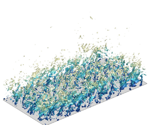
The dilatational components of the streamwise and wall-normal velocity fluctuations are reported in figure 9. In case M6-S, the fluctuations of $u''^d_t$ and $v''^d_t$ in the wall-parallel plane near the wall are organized in the form of streamwise positive–negative-alternating structures lying primarily within the low-speed streaks, namely the ‘travelling wave packets’ (TWPs), which were originally identified in hypersonic turbulent channel flows (Yu et al. 2019; Yu & Xu 2021) and boundary layers. In the vertical planes, these dilatational velocity fluctuations are fine structures inclined downstream. Although not strong enough to be manifested as shocklets (as will be shown later in § 5), they are indeed inherently small-scale motions compared with the solenoidal components. For this smooth wall case, their magnitudes are a decade smaller than those of the solenoidal components, suggesting their insignificant role in the flow dynamics, at least for the presently considered high-speed flows over adiabatic walls. For cases M6-R1 and M6-R2, the TWPs are also observed in the wall-parallel plane near the wall and are enhanced compared with case M6-S. In the vertical planes, the structures are inclined forward and bear a certain resemblance to those in case M6-S, but with stronger intensities and comparatively larger length scales that are obviously associated with the wavelengths of the imposed wall disturbances. Considering that the dispersive motions are already removed, these structures are unsteady, probably caused by the nonlinear interactions between the dispersive and turbulent motions.

Figure 9. Instantaneous distribution of the dilatational velocity, (a,c,e) $u''^d_t$, (b,d, f) $v''^d_t$ of case (a,b) M6-S, (c,d) M6-R1, (e, f) M6-R2, the lower wall: $y^+=10$.

4.1. Decomposition of Reynolds stresses

We further evaluate the contribution of the dilatational motions to the Reynolds stress. With the Helmholtz decomposition, the turbulent portion of the Reynolds stress can be decomposed as

(4.5)\begin{equation} R^+_{u_{i,t},u_{j,t}} = \underbrace{\frac{\overline{\rho u''^s_{i,t}u''^s_{j,t}}}{\tau_w}}_{R^+_{u^s_{i,t},u^s_{j,t}}} + \underbrace{\frac{\overline{\rho u''^s_{i,t}u''^d_{j,t}}}{\tau_w}}_{R^+_{u^s_{i,t},u^d_{j,t}}} + \underbrace{\frac{\overline{\rho u''^d_{i,t}u''^s_{j,t}}}{\tau_w}}_{R^+_{u^d_{i,t},u^s_{j,t}}} + \underbrace{\frac{\overline{\rho u''^d_{i,t}u''^d_{j,t}}}{\tau_w}}_{R^+_{u^d_{i,t},u^d_{j,t}}}. \end{equation}

The decomposed streamwise Reynolds normal stresses are shown in figure 10. For all the cases considered, the solenoidal components are the most intense. In cases S with smooth walls, neither the dilatational component nor the cross-correlations are significant, with their maximal values being no more than $0.01\,\%$ of the solenoidal component. With the wall disturbances, the intensities of the dilatational components are enhanced, but they are still lower by at least two orders than the solenoidal component. The cross-correlations between the solenoidal and dilatational components manifest a complex trend of variation, showing multiple peaks and valleys, the values of which are also trivial. These conclusions also apply to the spanwise component, therefore omitted here for brevity.

Figure 10. Wall-normal distribution of the decomposed Reynolds stress $R^+_{uu,t}$, (a–c) solenoidal components $R^+_{u^s_t u^s_t}$, (d–f) dilatational components $R^+_{u^d_t u^d_t}$, (g–i) correlations between the solenoidal and dilatational components $2R^+_{u^s_t u^d_t}$, (a,d,g) cases S, (b,e,h) cases R1, (c,f,i) cases R2. Line legends refer to table 1.

The decomposed wall-normal Reynolds normal stresses are shown in figure 11. For the smooth wall cases S, the dilatational components are negligible compared with the solenoidal components, but their cross-correlations constitute approximately $10\,\%$ of the total turbulent stress $R^+_{vv,t}$ at the highest Mach number considered here. In cases R1 and R2, the intensities of the dilatational component reach approximately $10\,\%$ of those in the solenoidal component at $M_\infty = 6$, with the maxima located at $y \approx 0.1 \delta$ in cases R1 and $y \approx 0.2 \delta$ in cases R2. Such intensification of the dilatational Reynolds stress component is mostly compensated by the negative cross-correlations, so the overall contribution related to the dilatational components remains low level. In the free stream, however, only the dilatational components contribute significantly to the velocity fluctuation intensities, whereas the solenoidal components are trivial in comparison, proving that the fluctuations in the free stream are primarily the dilatational motions related to the radiated acoustic waves from the boundary layer (Duan, Choudhari & Wu 2014; Duan, Choudhari & Zhang 2016) without significant vortices.

Figure 11. Wall-normal distribution of the decomposed Reynolds stress $R^+_{vv,t}$, (a–c) solenoidal components $R^+_{v^s_t v^s_t}$, (d–f) dilatational components $R^+_{v^d_t v^d_t}$, (g–i) correlations between the solenoidal and dilatational components $2R^+_{v^s_t v^d_t}$, (a,d,g) cases S, (b,e,h) cases R1, (c,f,i) cases R2. Line legends refer to table 1.

In figure 12 we present the components of the Reynolds shear stress. For the smooth wall cases S, the contribution of the dilatational components to the Reynolds shear stress is sufficiently small to be neglected, whereas the cross-correlation between the solenoidal and dilatational components contributes negatively by approximately $10\,\%$ in the near-wall region at $M_\infty = 6$. This is consistent with our previous findings in turbulent channel flows (Yu et al. 2019) at the centreline Mach number of $7$. The wall disturbances enhance the contribution of the dilatational component to approximately $5\,\%$ and in the meantime reduce that of the cross-correlation between solenoidal and dilatational motions. We can infer from this reduction in the cross-correlation that the physical processes of solenoidal and dilatational motions in the presence of wall disturbances are probably different in nature and their interactions are weak dynamically, at any rate where only the single-point statistics are concerned.

Figure 12. Wall-normal distribution of the decomposed Reynolds stress $-R^+_{uv,t}$, (a–c) solenoidal components $-R^+_{u^s_t v^s_t}$, (d–f) dilatational components $-R^+_{u^d_t v^d_t}$, (g–i) correlations between the solenoidal and dilatational components $-R^+_{u^s_t v^d_t}-R^+_{u^d_t v^s_t}$, (a,d,g) cases S, (b,e,h) cases R1, (c,f,i) cases R2. Line legends refer to table 1.

Lastly, we consider the contribution of the dilatational-related Reynolds shear stress to the skin friction. The most adopted method is the skin friction decomposition formula proposed by Fukagata, Iwamoto & Kasagi (2002), known as the ‘FIK’ identity, which is obtained by the trifold integration of the mean momentum equation, thereby decomposing the skin friction into the terms related to the viscous stress, Reynolds stress and, in boundary layers, the spatial development and mean flow convection. It is further applied to compressible turbulent channel flows for the evaluation of compressibility effects caused by flow property variation (Gomez, Flutet & Sagaut 2009) and dilatational motions (Yu et al. 2019). However, the trifold integration adopted in deriving the FIK identity has been criticized recently as lacking proper physical interpretation (Wenzel et al. 2022). Therefore, in the present study, the twofold integration proposed in the study of Wenzel et al. (2022) is used for better illustration of physical significance, written as

(4.6)\begin{equation} C_f = \underbrace{\frac{2}{\rho_\infty U^2_\infty \delta} \int^\delta_0 \tau_{xy} \,{\rm d}\kern0.05em y}_{C_V} - \underbrace{\frac{2}{\rho_\infty U^2_\infty \delta} \int^\delta_0 \overline{\rho u'' v''} \,{\rm d}\kern0.05em y}_{C_R} + \underbrace{\frac{2}{\rho_\infty U^2_\infty \delta} \int^\delta_0 (y-\delta) I_{x} \,{\rm d}\kern0.05em y}_{C_G}, \end{equation}

with $I_x$ expressed as

(4.7)\begin{equation} I_x={-} \frac{\partial \bar \rho \tilde u \tilde u}{\partial x} - \frac{\partial \overline{\rho u'' u''}}{\partial x} - \frac{\partial \bar \rho \tilde u \tilde v}{\partial y} - \frac{\partial \bar p}{\partial x} + \frac{\partial \bar \tau_{xx}}{\partial x}. \end{equation}

The $C_V$ and $C_G$ terms represent the contribution of viscous stress and spatial development and mean flow convection to the skin friction. The $C_R$ term originates from the contribution of the Reynolds stress which, by splitting it into the dispersive and turbulent stresses and the latter further into the solenoidal and dilatational components, can be further decomposed as

(4.8a,b)\begin{equation} C_R = C_{R,d} + C_{R,t},\quad C_{R,t}=C_{R,ts} + C_{R,td} + C_{R,tsd}. \end{equation}

The terms $C_{R,d}$ and $C_{R,t}$ denote the contributions of the dispersive and turbulent portions and $C_{R,ts}$, $C_{R,td}$ and $C_{R,tsd}$ those of the solenoidal, dilatational components and their cross-correlations. The expressions of these terms are similar to $C_{R,t}$ except that the velocity fluctuations are substituted by the corresponding velocity components.

Figure 13 reports the contributions of the terms in (4.6) to skin friction. The viscous stress and spatial development contribute to the skin friction by approximately $5\,\%$ and $38\,\%$ for cases with smooth walls and decrease slightly for cases with wall disturbances. Their abatement is compensated by the rising percentage of the $C_{R}$ related to the Reynolds stress, which increases with both the Mach number and the wavelength of the wall disturbances. The dispersive portion of the Reynolds stress is only restricted close to the wall within the height of approximately the sandgrain roughness $k_s$, so their direct contribution to the skin friction in terms of mean momentum is comparatively small at less than $5\,\%$ for the presently considered cases. The turbulent portion of the Reynolds stress is mostly constituted of the solenoidal component. The contribution of the dilatational component is positive and increases with the Mach number but is mitigated by the negative contribution of the cross-correlation between the solenoidal and dilatational velocities. For most of the cases, the terms related to the cross-correlation $C_{R,tsd}$ are greater than the genuine dilatational term $C_{R,td}$, but this is reversed for case M6-R2 where the latter surpasses the former in magnitude. In conclusion, in the integral sense of mean momentum balance, the contribution of the dilatational motions to the skin friction can be disregarded due to its insignificant value, despite their intensification in magnitude.

Figure 13. Contribution of each term in (4.6) to the skin friction.

4.2. Transport of turbulent kinetic energy

The intensification of the dilatational motions will also lead to the variation of turbulent kinetic energy transport. As we have shown in our previous study (Yu et al. 2023a), the dispersive portion of the fluctuations only have a strong impact on the budget terms in the near-wall region and our preliminary examination also suggests their weak Mach number dependence (not shown here for brevity). Henceforth, we only present the production and dissipation terms of the turbulent portion in this subsection.

By substituting the Helmholtz decomposition into the expression of turbulent kinetic energy (TKE) production, we have

(4.9)\begin{align} P_{K,t}&=P_{K,ts} + P_{K,td} + P_{K,tsd}\nonumber\\ & ={-}\overline{\rho u''^s_t v''^s_t} \frac{\partial \tilde u}{\partial y} -\overline{\rho u''^d_t v''^d_t} \frac{\partial \tilde u}{\partial y} -( \overline{\rho u''^s_t v''^d_t} + \overline{\rho u''^d_t v''^s_t} ) \frac{\partial \tilde u}{\partial y}. \end{align}

As shown in the left column of figure 14, the dilatational components $P_{K,td}$ are much smaller than the solenoidal ones for all the cases considered. The cross-correlation terms $P_{K,tsd}$ are approximately a decade smaller than the solenoidal component with the inclination of decreasing the turbulent TKE production.

Figure 14. Budget terms of turbulent kinetic energy, turbulent portion of (a,c,e) production term,(b,d, f) dissipation term, (a,b) cases S, (c,d) cases R1, (e, f) cases R2. Blue lines, cases M2; red lines, cases M4; black lines, cases M6. Symbols: original solid lines, solenoidal components; dashed lines, dilatational components; dash-dotted lines, cross-correlation.

The dissipation term can be decomposed by reformulating it as vorticity and divergence (Duan et al. 2011), i.e.

(4.10)\begin{equation} \varepsilon_t = \varepsilon_{t,s} + \varepsilon_{t,d} ={-} \overline{\mu \omega'_{i,t} \omega'_{i,t}} - \tfrac{4}{3} \overline{\mu \theta'_t \theta'_t}. \end{equation}

As shown in the right column of figure 14, the viscous dissipation caused by the vorticity $\varepsilon _{t,s}$ is at least ten times greater than that by divergence $\varepsilon _{t,d}$ within the boundary layer, whereas in the free stream this trend is reversed. It has been estimated in compressible isotropic turbulence that the ratio between them $\varepsilon _{t,d}/\varepsilon _{t,s}$ increases with the turbulent Mach number as a function of $M^4_t$, i.e.

(4.11)\begin{equation} \varepsilon_d \approx C_{\varepsilon} M^4_t \varepsilon_s. \end{equation}

In turbulent boundary layers, however, such patterns are difficult to find due to the statistical inhomogeneity in the wall-normal direction, but as has been shown by Duan et al. (2011), this estimation still holds at the locations where the turbulent Mach number $M_t$ reaches maxima. This is also validated with our presently obtained DNS databases, as shown in figure 15, except that the coefficient $C_{\varepsilon }$ seems higher for cases with wall disturbances, suggesting that the intensified dilatational motions by wall disturbances enhance the viscous dissipation.

Figure 15. Ratio between dilatational and solenoidal dissipation $\varepsilon _{t,d}/\varepsilon _{t,s}$. Line legends refer to table 1.

5. Strong compressive structures

Figure 9 shows that the dilatational velocity fluctuations are organized as sheet-like structures, enhanced by the wall disturbances. These structures are reminiscent of the shocklets in compressible isotropic (Lee, Lele & Moin 1991; Samtaney, Pullin & Kosović 2001; Wang et al. 2017, 2018) and homogeneous shear turbulence (Chen et al. 2018, 2019) at sufficiently high Mach numbers, namely the small-scale shock-like structures gradually appearing and occupying higher volume fractions of the flow. In wall-bounded turbulence, however, such structures are rarely observed, for the regions of high Mach number (near the free stream) and high turbulent intensities (close to the wall) are usually separated. The study of Duan et al. (2011) has shown, in hypersonic turbulence at the free-stream Mach number of $12$, possible evidence of the existence of eddy shocklets with numerical Schlieren and velocity divergence but lacks strict proof thereof, such as verifying whether the flow quantities on the two sides of the shocklets satisfy the Rankine–Hugoniot relation. In supersonic turbulent channel flows with sinuously distributed rough walls, it has been shown that the two-dimensional roughness is more sufficient in compressing the flow and that the quasi-steady shock waves have significant impacts on the flow statistics at the Mach number of $3.0$ (Tyson & Sandham 2013; Sun et al. 2018), whereas the three-dimensional roughness inclines to generate small-scale randomly oriented structures, which were assumed to be eddy shocklets (Jouybari et al. 2020). The cases with wall disturbances considered in the present study are similar to such a kind of three-dimensional roughness that induces the mean streamline curvature and hence the local flow compression and expansion. Since they are crucial to the flow dynamics and turbulent modelling, as we have demonstrated previously, in this section, we set out to identify the existence and nature of these shock-like structures and their variation with the Mach number.

A direct method of detecting the flow compression is to search for the regions where the velocity divergence $\theta '$ is strongly negative, but it lacks the capability of identifying their nature, i.e. whether they are the real shocklets. The previous experimental studies (Ekoto et al. 2009; Peltier et al. 2016) showed that the wall disturbances generally produce forward-inclined structures through which the fluid suffers compression as it travels downstream. Based on this feature, we only consider such the strong compressive events under the condition of both the strongly negative velocity divergence $\theta '_t < - 0.1 U_\infty / \delta$ and the positive streamwise pressure gradient $\partial p'/\partial x > p_\infty / \delta$ (see figure 16), with the former distinguishing the strong compression and the latter separating the shocklets from the rest of the identified structures. The pressure and density on the right and left sides of these structures are denoted as $p_r$, $\rho _r$ and $p_l$, $\rho _l$, respectively.

Figure 16. Illustration of the identification of compressive events.

In figure 17 we plot the probability density function (PDF) of $p_r/p_l$ against $\rho _r/\rho _l$ across the strong flow compression events inside the boundary layer. Three auxiliary lines highlighting the isothermal, shock and isentropic processes are shown. Note that, for the presently considered flow configuration, the relation between the pressure and density ratios in isentropic processes and shock waves show trivial deviations for the lack of extremely strong flow compression. For cases S with smooth walls, they exhibit no tendency of the strong compressive events falling on either curve, suggesting that the probability of the occurrence of shocklets is extremely low and that the pressure fluctuations are probably associated with vortical motions rather than thermodynamic processes.

Figure 17. Probability density function distribution of $p_r/p_l$ against $\rho _r/\rho _l$, (a) case M2-S, (b) case M2-R1,(c) case M2-R2, (d) case M4-S, (e) case M4-R1, ( f) case M4-R2, (g) case M6-S, (h) case M6-R1, (i) case M6-R2. Contour levels: $0.001 \sim 1.0$ with 7 equally distributed levels logarithmically. Blue lines, isothermal relation; green lines, Rankine–Hugoniot shock relation; red lines, isentropic relation.

The wall disturbances significantly alter the identified flow structures, especially in the relation between $p_r/p_l$ and $\rho _r/\rho _l$. For the cases at the free-stream Mach number of $2.0$, there is an inclination of the ratios of pressure and density on the right and left sides of the compressive events $p_r/p_l$ and $\rho _r/\rho _l$ falling on the curve of the isothermal relation. This suggests that the introduced wall disturbances at $M_\infty = 2$ are comparatively mild without inducing strong fluctuations of internal energy. At higher Mach numbers of $4.0$, the tendency of the ratios $p_r/p_l$ and $\rho _r/\rho _l$ falling on the isothermal relation is still there, but the probability of occurrence is higher for isentropic processes or shock waves which, at the free-stream Mach of $6.0$, are the dominant compressive events. Compared with cases R1, cases R2 with larger wavelengths show a higher probability of the occurrence of isothermal processes. This is justifiable because the compressive events are usually fine structures (Samtaney et al. 2001; Wang et al. 2017), which are more likely to be generated by wall disturbances with smaller wavelengths. In other words, the smaller wavelengths affect the dilatational motions and thermodynamic processes that are related to the fluctuations of internal energy more sufficiently. The wall disturbances with larger wavelengths, on the other hand, are prone to having stronger impacts on vortical and shear motions, as suggested by the enhanced Reynolds stress in figure 10.

Figure 18 shows the pressure fluctuations (the left column) at the free-stream Mach number of $6$ along with the identified strong flow compressive events under the condition of $\rho _r/\rho _l > 1.1$ and $p_r/p_l > (\rho _r/\rho _l)^{1.4}$ (lines in the left columns and isosurfaces in the right column). The criterion of the density ratio is chosen via the percolation analysis as the value when the volume of compressive events in the free stream, which is promised to be the weak isentropic processes, decreases to an insignificant value. With this criterion, the strong compressive events are barely observable in case M6-S, but in cases M6-R1 and M6-R2 with wall disturbances, the pressure fluctuations near the wall are intensified, related to the flow compression due to the mean streamline curvature. These compressive events generated on the wall travel to higher wall-normal locations and, due to the mean flow convection, inclined towards the downstream direction and manifested in the shape of sheets, as with those observed in isotropic turbulence (Samtaney et al. 2001; Wang et al. 2017). Notably, although the pressure fluctuations inside the boundary layers are stronger in case M6-R2 than those in case M6-R1, the induced compressive events are less in volume and weaker in strength, which should probably be ascribed to the larger wavelengths of the wall disturbances that alleviate the high pressure gradients in the streamwise direction. The implication is that the wall disturbances with larger wavelengths induce stronger vortex shedding but weaker flow compression, consistent with our previous presumption observed from the PDF in figure 17.

Figure 18. Instantaneous distribution of (a,c,e) pressure fluctuations (contours) and compressive events with $\rho _r/\rho _l > 1.1$ and $p_r/p_l = (\rho _r/\rho _l)^{1.4}$ (lines). (b,d, f) Compressive events, coloured by the wall-normal coordinate ($y/\delta$). (a,b) Case M6-S, (c,d) case M6-R1, (e, f) case M6-R2.

With the aid of the PDF and the flow visualizations in the instantaneous fields, we proved that there are barely any shocklets in the flow over smooth walls under the flow parameters considered herein. Only when the wall disturbances are introduced will there be comparatively strong compressive structures in the form of forward-inclined sheets in hypersonic flows, the structures that resemble the eddy shocklets in the compressible isotropic and homogeneous shear turbulence. However, they are not strong enough for us to distinguish whether they follow the patterns of isentropic or shock waves.

6. Conclusions

In the present study, we investigate the effects of wall disturbances, designed to emulate the imperfections of the fuselage of high-speed vehicles that induce the mean streamline curvatures, on the compressibility effects in supersonic and hypersonic turbulent boundary layers by exploiting DNS databases at Mach numbers up to 6. The turbulent and fluctuating Mach numbers, the intensity of density fluctuations and the velocity divergence suggest the more prominent compressibility effects in supersonic and hypersonic turbulence in the presence of wall disturbances. The streamwise fluctuating mass flux, i.e. the difference between the Favre and the Reynolds average of the velocity, is found to increase approximately linearly with the square of the turbulent Mach number and reach maxima of $9\,\%$ of the mean velocity close to the wall. The Favre- and Reynolds-averaged kinetic energy and Reynolds shear stress differ by approximately 30 % near the edge of the boundary layer at the free-stream Mach number of $6$ with the wall disturbances, suggesting the probable invalidation of Morkovin's hypothesis that assumes the insignificance of the density fluctuations in the flow dynamics.

We further split the velocity fluctuations into the solenoidal, rotational and potential, dilatational portions using the Helmholtz decomposition. The instantaneous velocity distribution of the former resembles those of the incompressible flows and that of the latter is organized as TWPs in the wall-parallel plane and downstream-inclined radiated waves. Although the dilatational fluctuations are stronger for the cases with wall disturbances at the Mach number of $6$, their contributions to the Reynolds stress and the skin friction are still negligible. So are their roles in the production of the turbulent kinetic energy, but the viscous dissipation is enhanced, proportional to $M^4_t$.

The PDF of the ratio of pressure and density on the two sides of the compressive events shows that there are barely any shocklets in smooth wall turbulence, even at the highest Mach number. With the presence of the wall disturbances, the strong compressive events show more of a tendency of being isothermal processes at the Mach number of $2$ where the wall disturbances are not strong enough to induce the fluctuation of the internal energy, whereas at higher Mach numbers the strong compressive events incline to follow either the isentropic or the Rankine–Hugoniot relation, the disparity between which is not evident due to the comparatively weak intensity of flow compression. Moreover, the wall disturbances with shorter wavelengths are prone to generating stronger compressive events.

Lastly, we would like to point out that the Reynolds number effects are not considered in the present study. The Reynolds numbers considered herein are comparatively low, especially for the turbulence over smooth walls, so the slight difference in the friction Reynolds number $Re_\tau$ will probably lead to obvious deviations in the turbulent statistics. Obtaining quantitative scaling laws regarding the mean and fluctuating velocities requires more precise control of the flow parameters. However, the conclusions obtained herein will not be altered, for most of them are based on the comparison between the dilatational and solenoidal components or between the mean and fluctuating velocities in each case without incorporating the effects of Reynolds numbers.

The evaluation of the compressibility effects under the influences of wall disturbances is limited to quasi-adiabatic flows. As we have noticed in the paper, the dilatational motions are fine-scale structures that are more likely to play a significant role in viscous dissipation and increase the local temperature and hence the wall heat flux. Their contribution to the wall heat transfer will be considered in our future work.