Shear dispersion of multispecies electrolyte solutions in the channel domain

Abstract

In multispecies electrolyte solutions, even in the absence of an external electric field, differences in ion diffusivities induce an electric potential and generate additional fluxes for each species. This electro-diffusion process is well-described by the advection Nernst–Planck equation. This study aims to analyse the long-time behaviour of the governing equation under electroneutrality and zero current conditions, and to investigate how the diffusion-induced electric potential and shear flow enhance the effective diffusion coefficients of each species in channel domains. The exact solutions of the effective equation with certain special parameters, as well as the asymptotic analyses for ions with large diffusivity discrepancies, are presented. Furthermore, there are several interesting properties of the effective equation. First, it is a generalization of the Taylor dispersion, with a nonlinear diffusion tensor replacing the scalar diffusion coefficient. Second, the effective equation exhibits a scaling relation, revealing that the system with a weak flow is equivalent to the system with a strong flow under scaled physical parameters. Third, in the case of injecting an electrolyte solution into a channel containing well-mixed buffer solutions or electrolyte solutions with the same ion species, if the concentration of the injected solution is lower than that of the pre-existing solution, then the effective equation simplifies to a multi-dimensional diffusion equation. However, when introducing the electrolyte solution into a channel filled with deionized water, the ion–electric interaction results in several phenomena not present in the advection–diffusion equation, including upstream migration of some species, spontaneous separation of ions, and non-monotonic dependence of the effective diffusivity on Péclet numbers. Finally, the dependence of effective diffusivity on concentration and ion diffusivity suggests a method to infer the concentration ratio of each component and ion diffusivity by measuring the effective diffusivity.

1. Introduction

Fluid flow plays an important role in the transport of solutes. When a solute is transported in a fluid through a narrow tube or channel, the interaction of fluid flow and molecular diffusion causes the solute to spread out and become more dispersed as it travels down the tube. This effect is known as Taylor dispersion, named after G.I. Taylor, who first investigated the phenomenon in Taylor (1953). Since Taylor's seminal work, theoretical studies on Taylor dispersion have exploded in many directions (Aris 1956, 1960; Chatwin 1970; Vedel & Bruus 2012; Ding & McLaughlin 2022a) and established applications in many disciplines, such as molecular diffusivity measurement (Bello, Rezzonico & Righetti 1994; Leaist 2017; Taladriz-Blanco et al. 2019), chemical delivery in micro-channels (Dutta & Leighton 2001; Aminian et al. 2016) and contaminant dispersion (Chatwin 1975; Smith 1982; Ngo-Cong et al. 2015).

In an electrolyte solution, the electric current is carried by the dissolved ions. The electric field exerts significant body forces on the ions, affecting their fluxes, which is another key factor in mass transfer. Even in the absence of an external electric field, where the electroneutrality and zero current conditions are met, it is necessary to consider ion–electric interaction in multispecies electrolyte solutions because dissolved ions have different diffusivities. To maintain electroneutrality, the faster-moving ion is slowed down, creating a balance between positive and negative charges. For example, sodium fluorescein is a tracer used commonly in fluid experiments, and its self-diffusion coefficient in water has been measured experimentally by several authors to be approximately $4\unicode{x2013}5\times 10^{-6}\ {\rm cm}^{2}\ {\rm s}^{-1}$ (Casalini et al. 2011). However, in a sodium chloride stratified fluid, the diffusion coefficient of sodium fluorescein could exhibit a significant increase, reaching values $8\unicode{x2013}9\times 10^{-6}\ {\rm cm}^{2}\ {\rm s}^{-1}$ (Ding et al. 2021).

The system involves fluid flow, electric field diffusion, and can be well-described by the advection Nernst–Planck equation (Deen 1998; Lyklema 2005; Cussler 2013). Many recent studies show that the transport of multiple electrolytes exhibits different properties compared with the transport of a single binary electrolyte (Hosokawa et al. 2011; Liu, Shang & Zachara 2011; Gupta et al. 2019). When dealing with two different ion species, the nonlinear governing equation can be reduced to the advection–diffusion equation (Deen 1998), allowing for simplified analysis. However, when dealing with more than two different ion species, the complexity of the nonlinear governing equation prohibits simplification to the advection–diffusion equation, necessitating a comprehensive consideration of the electro-diffusive process to describe the system's behaviour accurately.

Understanding how fluid flow, electric potential and diffusion interact in multispecies electrolyte solutions is essential for measuring accurately mutual diffusion (Price 1988; Leaist & Hao 1993; Ribeiro et al. 2019; Rodrigo et al. 2021, 2022), as well as for simulating the system with stratified fluids (Ben-Yaakov 1972; Yuan-Hui & Gregory 1974; Poisson & Papaud 1983; Ding et al. 2021; Ding & McLaughlin 2023), and for controlling diffusiophoresis (Ault et al. 2017; Alessio et al. 2022) and modelling isotachophoresis (Bhattacharyya et al. 2013; Gopmandal & Bhattacharyya 2015; GanOr, Rubin & Bercovici 2015) and chromatography (Biagioni, Cerbelli & Desmet 2022). Despite its importance, the interplay between these three factors has not been studied extensively in the literature, creating a knowledge gap. The main goal of this study is to fill this gap by presenting a comprehensive investigation of this interplay.

To this end, we use homogenization methods to derive an effective equation that is valid at the diffusion time scale for the advection Nernst–Planck equation in a channel with arbitrary cross-sectional geometry. In addition, the resulting effective equation depends only on the longitudinal variable of the channel, and provides a more tractable approximation for analysing mass transfer that captures the combined effects of flow advection and ion–electric interaction. Our analysis of the effective equation shows that the variance of the concentration distribution increases asymptotically linearly with time, and we demonstrate that the effective diffusivity can be calculated efficiently via the self-similar solution of the effective equation. Effective diffusivity is a critical parameter for understanding the mass transfer and guiding the designing of microfluidic devices (Dutta & Leighton 2001), and we show that it can also be used to infer the concentration ratio of each component and ion diffusivity in multispecies electrolyte solutions. We demonstrate that the effective equation exhibits a reciprocal property, namely, the system without flow is mathematically equivalent to the system with a strong flow and scaled physical parameters. We derive the self-similarity solution of the effective equation and present asymptotic analyses for ions with large diffusivity discrepancies. Moreover, we find that the nonlinear effective equation can be approximated by a diffusion equation with mutual diffusion coefficients when the background concentration is non-zero, consistent with previous studies (Rodrigo et al. 2022).

To complement our analytical results, we conduct numerical simulations to explore the behaviour of multispecies electrolyte solutions under different flow and electric field conditions, validating our analytical results. Our simulations reveal several interesting properties arising from the nonlinearity of the advection Nernst–Planck equation, such as upstream migration of some species, separation of ions depending on the flow strength, the presence of highly non-Gaussian and bimodal shapes of concentration distribution, and a non-monotonic dependence of the effective diffusivity on Péclet numbers.

The paper is organized as follows. In § 2, we introduce the governing equations for the transport of multispecies electrolyte solutions in channel domains and provide a comprehensive overview of effective diffusivity. Section 3 presents the derivation of the effective equation for the advection Nernst–Planck equation at long times using homogenization methods. In § 3.2, we outline the effective equation for specific shear flows in parallel-plate channel domains and circular pipes. Section 3.3 discusses the self-similarity solution for different types of initial conditions, and presents the formula for calculating the effective diffusivity using this solution. Section 3.4 compares our results with those of Taylor dispersion, and highlights the reciprocal property exhibited by the effective equation. In § 4, we provide the exact solution of the effective equation for certain parameter combinations, and analyse cases with significant differences in ion diffusivity. Section 5 validates our analytical results through numerical simulations, and explores intriguing phenomena resulting from ion–electric interactions. Finally, in § 6, we summarize our findings and discuss potential avenues for future research.

2. Governing equation and effective diffusivity

2.1. Advection Nernst–Planck equation

We consider the electrolyte solution transport in a channel domain: $(x, \boldsymbol {y}) \in \mathbb {R}\times \varOmega$, where the $x$-direction is the longitudinal direction of the channel, and $\varOmega \subset \mathbb {R}^{d}$ stands for the cross-section of the channel. Here, $\boldsymbol {n}$ is the outward normal vector of the boundary $\mathbb {R} \times \partial \varOmega$, where $\partial \varOmega$ is the boundary of $\varOmega$. Some practical examples of the channel boundary geometry include the parallel-plate channel $\varOmega = \{ y\,|\,y \in [0,L_{y}] \}$ (sketched in figure 1), the circular pipe $\varOmega =\{ \boldsymbol {y}\,|\,\boldsymbol {y}^{2}\leqslant L_{y}^{2} \}$, the rectangular duct $\varOmega =\{ \boldsymbol {y}\,|\,\boldsymbol {y} \in [0,L_{y}]\times [0,H_{y}] \}$, and bowed rectangular channels (Lee et al. 2021).

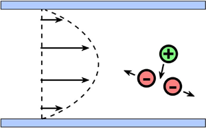
Figure 1. The schematic shows the set-up for the special case of a quadratic shear flow in the parallel-plate channel domain. A multispecies electrolyte in water exists in the form of dissolved ions. Ions of like charges repel, while ions of opposite charges attract, due to electrostatic forces. The interplay between the flow and the ion–electric interactions has a crucial role in determining the behaviour and dynamics of the system.

Denote the concentration and valence of the $i$th species of ion as $c_{i} (x,\boldsymbol {y},t)$ and $z_i$, respectively. The concentration evolution of $n$ ion species under the shear flow advection and ionic interaction can be modelled by the Nernst–Planck equation (see § 11.7 in Deen (1998), or Maex (2013))

(2.1)\begin{align} \partial_{t}c_{i}+\boldsymbol{\nabla}\boldsymbol{\cdot} \left( \boldsymbol{u} c_{i} \right)=\kappa_{i}\,\Delta c_{i}+ \frac{\kappa_{i} z_{i} e }{k_{B} T}\, \boldsymbol{\nabla}\boldsymbol{\cdot}(c_{i}\,\boldsymbol{\nabla}\phi),\quad c_{i} (x,\boldsymbol{y},0)=c_{I,i} \left( \frac{x}{L_{x}}\right), \quad i=1,\dots,n, \end{align}

where $\kappa _{i}$ is the diffusivity of the $i$th species of ion, $\phi (x,\boldsymbol {y},t)$ is the electric potential, $e$ is the elementary charge, $k_B$ is the Boltzmann constant, $T$ is the temperature, $c_{I,i}$ is the initial condition of the $i$th species of ion, and $L_{x}$ is the characteristic length scale of the initial condition. The second term on the left-hand side of (2.1) describes the fluid flow advection. The first term on the right-hand side of (2.1) describes the ion diffusive motion, while the second term represents the electromigration in response to the local electric field.

We assume that the electrolyte solutions are advected passively by a prescribed velocity field that takes the form $\boldsymbol {u} = (u (\boldsymbol {y},t), 0, \dots, 0)$. The function $u (\boldsymbol {y},t)$ vanishes on the boundary wall and exhibits periodic time-varying behaviour with period $L_{t}$. While steady pressure-driven flow is common in many applications (Price 1988; Leaist & Hao 1993; Rodrigo et al. 2021), we maintain the general form and time dependence of the flow to ensure the theoretical framework's applicability to various scenarios, including blood flow (Marbach & Alim 2019) and scalar intermittency (Majda & Kramer 1999; Camassa et al. 2021). We impose the no-flux boundary condition for the concentration fields of the ion species $\boldsymbol {n}\boldsymbol {\cdot }(\kappa _{i}\,\boldsymbol {\nabla } c_{i} + ({\kappa _{i} z_{i} e }/{k_{B} T}) c_{i}\,\boldsymbol {\nabla }\phi ) |_{\mathbb {R}\times \partial \varOmega }=0$.

Now there are $n$ conservation equations for $n$ concentration fields, and an unknown electric potential $\phi$. An additional Poisson equation can be derived from Gauss’ law, which is one of Maxwell's equations of electricity and magnetism. When combined with the Nernst–Planck equation, it forms the Poisson–Nernst–Planck system (Schmuck & Bazant 2015). However, this work focuses on the case in the absence of an external electric field. The net charge density is zero almost everywhere. We consider two alternative equations that serve as reasonable approximations of the Poisson equation in this setting. The first additional equation arises from the electroneutrality condition $\sum _{i=1}^{n} z_{i}c_{i}=0$. The second condition is the zero electric current condition, given by

(2.2)\begin{equation} \boldsymbol{0}= \sum_{i=1}^{n}z_{i}\boldsymbol{J}_{i}=\sum_{i=1}^{n}z_{i} \left(\boldsymbol{u} c_{i}- \kappa_{i}\,\boldsymbol{\nabla} c_{i}- \frac{\kappa_{i}z_{i} e }{k_B T}\,c_{i}\,\boldsymbol{\nabla} \phi \right), \end{equation}

which is used commonly in the literature when there is no external electric field (Ben-Yaakov 1972; Gupta et al. 2019; Tournassat, Steefel & Gimmi 2020; Tabrizinejadas et al. 2021). Moreover, for the electroneutrality initial data, the zero electric current condition ensures that the electroneutrality condition is always true (see Boudreau, Meysman & Middelburg 2004).

Using the zero electric current condition, the gradient of the electric potential can be expressed in terms of ion concentrations:

(2.3)\begin{equation} \frac{e }{k_BT}\,\boldsymbol{\nabla}\phi= \frac{\displaystyle\sum_{i=1}^{n}z_{i} \left(\boldsymbol{u}c_{i} - \kappa_{i}\, \boldsymbol{\nabla} c_{i} \right)}{\displaystyle\sum_{i=1}^{n}z_{i}^{2} \kappa_{i} c_{i} }= \frac{\displaystyle\sum_{i=1}^{n-1}(\kappa_{n}-\kappa_{i}) z_{i}\, \boldsymbol{\nabla}c_{i} }{\displaystyle\sum_{i=1}^{n-1} (z_{i} \kappa_{i}-z_{n}\kappa_{n})z_{i}c_{i} }, \end{equation}

where the second step follows the electroneutrality condition. Equation (2.3) shows that the electric potential gradient is induced by the difference in ion diffusivities. When all diffusivities take the same value, the gradient of the diffusion-induced potential becomes zero, and (2.1) reduces to the advection–diffusion equation. When there is a difference in diffusivities, substituting (2.3) into the Nernst–Planck equation (2.1) yields the equation that will be used mainly in this study:

(2.4)\begin{align} \partial_{t}c_{i}+u (\boldsymbol{y},t)\,\partial_{x} c_{i}=\kappa_{i}\,\Delta c_{i}+ \kappa_{i} z_{i}\, \boldsymbol{\nabla}\boldsymbol{\cdot}\left( \frac{ c_{i} \displaystyle\sum_{j=1}^{n-1} (\kappa_{n}- \kappa_{j}) z_{j}\, \boldsymbol{\nabla} c_{j} }{\displaystyle\sum_{j=1}^{n-1}(z_{j} \kappa_{j}-z_{n}\kappa_{n}) z_{j}c_{j} } \right), \quad i=1,\dots,n-1. \end{align}

This system of equations exhibits an interesting scaling property, wherein any solution multiplied by a constant remains a valid solution to the system. Furthermore, if all valences are multiplied by a constant, then the original solution of the system remains a solution to the system with the new valences.

We proceed by considering a combination of typical experimental physical parameters, aiming to identify the dominant factors in the problem and facilitate perturbation analysis. The diffusivity of the solute is approximately $10^{-5}\ {\rm cm}^{2}\ {\rm s}^{-1}$. The length scale of concentration, denoted as $L_{x}$, ranges from millimetres to centimetres. Meanwhile, the channel width, denoted as $L_{y}$, spans from micrometres to millimetres. As depicted in figure 2, the advection caused by flow and the diffusion contribute to the phenomenon, leading to the condition $L_{x}\gg L_{y}$. The characteristic fluid velocity varies from millimetres per second to centimetres per second. Additionally, apart from microfluidic experiments, our study also has implications for blood flow scenarios, where a rich variety of electrolytes are present. Depending on the type of blood vessel, typically their radii range from 10 to 200 micrometres, and blood velocities vary from $0.1$ to $20\ {\rm cm}\ {\rm s}^{-1}$.

Figure 2. Experimental photo showing the advection of a sodium fluorescein solution in a pipe through pressure-driven flow. The purple regions represent the presence of ultraviolet tube lights. Upon exposure to these lights, the sodium fluorescein solution emits a vibrant green light. The experimental set-up includes a pump attached to the left-hand end of the pipe, which generates a steady pressure-driven flow to transport the sodium fluorescein solution towards the right. For the detailed procedure and set-up of the laminar channel flow experiments, we refer to Aminian et al. (2018).

When an object's surface is exposed to a fluid, two parallel layers of charge surrounding the object appear. Specifically, under a strong applied electric field, electro-osmotic flow occurs (Ghosal & Chen 2012), which has numerous applications in microfluidics. One might question whether the assumptions of electroneutrality and zero current still hold in the presence of surface changes. However, in this study, we can neglect the effects of surface charge for the following reasons. First, the characteristic thickness of the double layer, known as the Debye length, is typically of the order of nanometres (Hashemi et al. 2018). This is significantly smaller than the characteristic width of the micro-channel, which ranges from micrometres to millimetres. Second, in the absence of an external electric field, electro-osmotic flow is negligible compared to the fluid flow imposed by other factors, such as the pressure-driven flow produced by the pump.

2.2. Effective diffusivity

As demonstrated by many studies (Taylor 1953; Aris 1956; Chatwin 1970; Ding & McLaughlin 2022b), the solution of the advection–diffusion equation in the channel domain converges to a Gaussian distribution function at long times. To model this behaviour, one can use a diffusion equation with an enhanced effective diffusion coefficient. Therefore, understanding the dependence of the effective diffusion coefficient on the flow conditions, channel geometries and ion physical parameters is important for optimizing microfluidic device performance, either enhancing or reducing mixing (Dutta & Leighton 2001; Aminian et al. 2015, 2016).

The precise definition of the effective diffusion coefficient depends on the initial condition. In this study, we consider three types of initial conditions. The first type is an integrable function that vanishes at infinity, such as $c_{I,i} (x) = ({2}/{\sqrt {{\rm \pi} }})\,{\rm e}^{-x^{2}}$. This type of initial condition can be used to model the delivery of chemicals with a finite volume in a capillary tube (see Aminian et al. 2016). In the second type of initial condition, the concentration field can be expressed as $c_{i} (x,\boldsymbol {y},t) =c_{i} (\infty )+ \tilde {c}_{i} (x,\boldsymbol {y},t)$, where $c_{i} (\infty )$ is a constant representing the background concentration, and $\tilde {c}_{i}$ is an integrable function representing the deviation from the background concentration, for example, $c_{I,i} (x) =1+({2}/{\sqrt {{\rm \pi} }})\,{\rm e}^{-x^{2}}$. In many experimental studies (e.g. Leaist & MacEwan 2001; Leaist 2017), the pipe is filled with buffer solutions. In such cases, $c_{i}(\infty )>0$, and $\tilde {c}_i$ can take negative values as long as $c_i$ remains non-negative. In the third type of initial condition, the concentration field tends to a constant value at infinity, but the values at positive and negative infinity can be different, such as $c_{I,i} (x) = \mathrm {erf} (x) =({2}/{\sqrt {{\rm \pi} }})\int _{0}^{x}{\rm e}^{-t^{2}}\,\mathrm {d}t$, which can be used to model the continuous injection of a solution with a constant concentration into the channel domain (see Taylor 1953). The solutions of the equations with these three types of initial conditions exhibit different long-time asymptotic properties, therefore we have treated them separately in our analysis.

For the first type of initial condition, the effective longitudinal effective diffusivity is given by

(2.5)\begin{equation} \kappa_{{eff},i}= \lim_{t\rightarrow \infty}\frac{\mathrm{Var} (\bar{c}_{i})}{2t\displaystyle\int_{-\infty}^{\infty} \bar{c}_{i}\,\mathrm{d}x}= \lim_{t\rightarrow \infty} \frac{\partial_{t}\,\mathrm{Var} (\bar{c}_{i})}{2 \displaystyle\int_{-\infty}^{\infty} \bar{c}_{i}\,\mathrm{d}x}, \end{equation}

where

(2.6)\begin{equation} \bar{c}_{i} (x,t) = \frac{1}{| \varOmega|}\int_{\varOmega}c_{i} (x,\boldsymbol{y},t) \,\mathrm{d}\boldsymbol{y} \end{equation}

is the cross-sectional average of the scalar field $c_{i}$. Here, $| \varOmega |$ is the area of $\varOmega$, and

(2.7)\begin{equation} \mathrm{Var} (\bar{c}_{i})= \int_{-\infty}^{\infty} \bar{c}_{i} x^{2}\,\mathrm{d}x-\left(\int_{-\infty}^{\infty} \bar{c}_{i} x\,\mathrm{d}x \right)^{2} \end{equation}

is the variance of the cross-sectional averaged concentration field $\bar {c}_{i}$. In other words, the asymptotics of the variance is given by

(2.8)\begin{equation} \mathrm{Var} (\bar{c}_{i}) \approx \mathrm{Var} (\bar{c}_{I,i})+ 2 t\,\kappa_{eff} \int_{-\infty}^{\infty} \bar{c}_{i}\,\mathrm{d}x, \quad t \rightarrow \infty. \end{equation}

For the second type of initial condition, where the background ion concentration is non-zero, $c_i$ is not integrable. One can define the effective longitudinal effective diffusivity via the perturbed concentration

(2.9)\begin{equation} \kappa_{{eff},i}= \lim_{t\rightarrow \infty}\frac{\mathrm{Var} (\bar{c}_{i}-c_{i} (\infty))}{2t \displaystyle\int_{-\infty}^{\infty} (\bar{c}_{i}-c_{i} (\infty))\,\mathrm{d}x} =\lim_{t\rightarrow \infty}\frac{\partial_{t}\,\mathrm{Var} (\bar{c}_{i}-c_{i} (\infty))}{2 \displaystyle\int_{-\infty}^{\infty} (\bar{c}_{i}-c_{i} (\infty))\,\mathrm{d}x}. \end{equation}

The solution with the third type of initial condition is also not integrable, but we can investigate its derivative:

(2.10)\begin{equation} \kappa_{{eff},i}= \lim_{t\rightarrow \infty}\frac{\mathrm{Var} (\partial_{x}\bar{c}_{i})}{2t (\bar{c}_{i} (\infty) -c_{i} (-\infty)) }= \lim_{t\rightarrow \infty}\frac{\partial_{t} \,\mathrm{Var} (\partial_{x}\bar{c}_{i})}{2 (\bar{c}_{i} (\infty) -c_{i} (-\infty))}. \end{equation}

Although the diffusion-induced electric potential may cause the concentration field to deviate from a Gaussian distribution function, we are still interested in computing the effective diffusivity for several reasons. First, when the electric potential is weak and the background concentration is non-zero, the solution can be approximated reasonably by a Gaussian distribution function or error function. Second, as the time approaches infinity, the longitudinal variance of the concentration field increases linearly, ensuring that the effective diffusivity remains a well-defined quantity for characterizing the system. Third, by examining the relationship between effective diffusivity and other physical parameters, e.g. ion diffusivity, one can devise an experimental method for measuring the latter.

3. Effective equation

It is possible to develop a simplified model that depends only on the longitudinal variable and time, given that the length scale in the longitudinal direction of the channel domain is significantly larger than the length scale in the transverse direction (as shown in figure 2). By simplifying the model in this way, one can reduce the computational complexity of the problem while retaining the relevant physical phenomena without compromising the key features of interest. The homogenization method is a method that is widely used to achieve this goal, especially for the linear advection–diffusion problem (Camassa, Lin & McLaughlin 2010; Wu & Chen 2014). Here, we will employ the homogenization method to derive the effective equation for the nonlinear equation (2.1).

3.1. Homogenization method

The first step is to non-dimensionalize the equation, which helps to identify the dominant terms. The change of variables for the non-dimensionalization is

(3.1)\begin{equation} \left.\begin{gathered} L_{x}x'=x,\quad L_{y}\boldsymbol{y}'=\boldsymbol{y}, \quad \epsilon= \frac{L_{y}}{L_{x}}, \quad \frac{L_{y}^{2}}{\tilde{\kappa} \epsilon^2}\,t'=t,\\ \tilde{c}c_{i}'=c_{i}, \quad \frac{e }{k_BT}\,\phi'=\phi,\quad Uu' \left( \boldsymbol{y}',\frac{t'}{\epsilon^{2}} \right)= u(\boldsymbol{y},t), \end{gathered}\right\} \end{equation}

where $\tilde {c}$ is the characteristic concentration, and $\tilde {\kappa }$ is the characteristic diffusivity. One can drop the primes without confusion and obtain the non-dimensionalized equation

(3.2)\begin{equation} \left.\begin{gathered} \partial_{t}c_{i}+\frac{{Pe}\,u \left( \boldsymbol{y}, \dfrac{t}{\epsilon^2} \right)}{\epsilon}\, \partial_{x} c_{i}=\kappa_{i} \partial_{x}( \partial_{x}c_{i}+z_{i}c_{i}\partial_{x}\phi )+ \frac{\kappa_{i} }{\epsilon^{2}}\,\boldsymbol{\nabla}_{\boldsymbol{y}} \boldsymbol{\cdot}\left(\boldsymbol{\nabla}_{\boldsymbol{y}}c_{i}+z_{i} c_{i}\, \boldsymbol{\nabla}_{\boldsymbol{y}}\phi \right),\\ \left. c_{i} \right|_{t=0}=c_{I,i} ( x ),\quad \left. \boldsymbol{n}\boldsymbol{\cdot}\kappa_{i} \left(\partial_{x}c_{i}+ \frac{1}{\epsilon}\,\boldsymbol{\nabla}_{\boldsymbol{y}} c_{i} + z_{i} c_{i} \left(\partial_{x}\phi + \frac{1}{\epsilon}\,\boldsymbol{\nabla}_{\boldsymbol{y}} \phi\right)\right) \right|_{\mathbb{R}\times \partial\varOmega }=0,\\ \qquad i=1,\dots,n-1,\\ \boldsymbol{\nabla}\phi= \frac{\displaystyle\sum_{i=1}^{n-1} (\kappa_{n}- \kappa_{i}) z_{i}\, \boldsymbol{\nabla}c_{i} }{\displaystyle\sum_{i=1}^{n-1} (z_{i} \kappa_{i}-z_{n}\kappa_{n})z_{i}c_{i} }, \end{gathered}\right\} \end{equation}

where $\boldsymbol {\nabla }_{\boldsymbol {y}}= ( \partial _{y_{1}}, \dots, \partial _{y_{d}} )$, ${Pe}={L_{y}U}/{\tilde {\kappa }}$ is the Péclet number, and $u (\boldsymbol {y},t)$ has a temporal period $\tilde {L}_{t}=\kappa L_{t}/L_{y}^{2}$. It is convenient to introduce two different scales in time: $t$ (slow) and $\tau = {t}/{\epsilon ^2}$ (fast). Consequently, the differential operators in time will be replaced $\partial _{t}\rightarrow \partial _{t}+({1}/{\epsilon ^{2}})\partial _{\tau }$, and the equation becomes

(3.3)\begin{align} \partial_{t}c_{i}+\frac{\partial_{\tau}c_{i}}{\epsilon^{2}}+\frac{Pe}{\epsilon}\,u ( \boldsymbol{y}, \tau )\,\partial_{x} c_{i}=\kappa_{i} \partial_{x}( \partial_{x}c_{i}+z_{i}c_{i} \partial_{x}\phi )+ \frac{\kappa_{i} }{\epsilon^{2}}\,\boldsymbol{\nabla}_{\boldsymbol{y}} \boldsymbol{\cdot}\left(\boldsymbol{\nabla}_{\boldsymbol{y}}c_{i}+z_{i} c_{i}\, \boldsymbol{\nabla}_{\boldsymbol{y}}\phi \right). \end{align}

Notice that the equation is invariant under the translation in $x$. For convenience, one can consider applying the Galilean transformation $\tilde {x}=x- \langle u (\boldsymbol {y},\tau ) \rangle _{\boldsymbol {y},\tau }\,t$ so that the resulting new shear flow $\tilde {u}=u- \langle u (\boldsymbol {y},\tau ) \rangle _{\boldsymbol {y},\tau }$ has a zero average, where the average of a function is defined as

(3.4)\begin{equation} \langle f (\boldsymbol{y},\tau)\rangle_{\boldsymbol{y},t}=\frac{1}{|\varOmega|\,\tilde{L}_{t}}\int_{\varOmega} \int_{0}^{\tilde{L}_{t}} f (\boldsymbol{y},\tau)\,\mathrm{d} \boldsymbol{y}\,\mathrm{d} \tau. \end{equation}

Assume that the asymptotic expansion of $c_{i}$ in the limit $\epsilon \rightarrow 0$ is

(3.5)\begin{equation} c_{i}(x,\boldsymbol{y},t)=c_{i,0}(x,y,t,\tau)+\epsilon\, c_{i,1}(x,y,t,\tau)+\epsilon^{2}\,c_{i,2}(x,y,t,\tau)+{O}(\epsilon^3). \end{equation}

Substituting the asymptotic expansion of $c_i$ into the formula for $\phi$ and using the Taylor expansion yields the asymptotic expansion of $\phi$, i.e. $\phi =\phi _{0}+\epsilon \phi _{1}+\epsilon ^{2} \phi _{2} +{O} (\epsilon ^{3})$. In particular, the gradients of the first two coefficients are given by

(3.6)\begin{align} \left.\begin{gathered} \boldsymbol{\nabla} \phi_{0}= \frac{\displaystyle\sum_{i=1}^{n-1} (\kappa_{n}- \kappa_{i}) z_{i}\, \boldsymbol{\nabla} c_{i,0} }{\displaystyle\sum_{i=1}^{n-1} (z_{i} \kappa_{i}-z_{n}\kappa_{n})z_{i}c_{i,0} },\\ \boldsymbol{\nabla}\phi_{1}= \frac{\displaystyle\sum_{i=1}^{n-1} (\kappa_{n}- \kappa_{i})z_{i}\, \boldsymbol{\nabla} c_{i,1} }{\displaystyle\sum_{i=1}^{n-1} (z_{i} \kappa_{i}-z_{n}\kappa_{n}) z_{i}c_{i,0} } + \frac{\left(\displaystyle\sum_{i=1}^{n-1}(\kappa_{n}- \kappa_{i}) z_{i}\, \boldsymbol{\nabla} c_{i,0} \right) \left( \displaystyle\sum_{i=1}^{n-1} (z_{i} \kappa_{i}-z_{n} \kappa_{n})z_{i}c_{i,1} \right)}{ \left(\displaystyle\sum_{i=1}^{n-1}(z_{i} \kappa_{i}-z_{n}\kappa_{n})z_{i}c_{i,0} \right)^{2}}. \end{gathered}\right\} \end{align}

Substituting the expansion of $c_i$ and $\boldsymbol {\nabla } \phi$ into (3.3) leads to an equation involving the power series of $\epsilon$. Since the equation holds for arbitrarily small $\epsilon$, the coefficient of each power of $\epsilon$ should be zero, which yields a hierarchy of equations for $c_{i,k}$.

Grouping all terms of order ${O}(\epsilon ^{-2})$ and setting the coefficient to be zero yields

(3.7a,b)\begin{equation} \partial_{\tau}c_{i,0}=\kappa_{i}\,\boldsymbol{\nabla}_{\boldsymbol{y}}\boldsymbol{\cdot} \left( \boldsymbol{\nabla}_{\boldsymbol{y}}c_{i,0}+z_{i} c_{i,0}\, \boldsymbol{\nabla}_{\boldsymbol{y}}\phi_{0} \right), \quad \left. c_{i,0} \right|_{t=0,\tau=0 }=c_{I,i} \left( x \right). \end{equation}

The initial condition is a function of the variable $x$ only, which means that $c_{i,0}(x,\boldsymbol {y},t,\tau )=c_{i,0}(x,t)$, $i=1, \dots,n$. Consequently, the evolution equation for $c_{i,0}$ provides the desired approximation. The goal of this homogenization calculation is to derive this equation.

Grouping all terms of order ${O}(\epsilon ^{-1})$ yields

(3.8)\begin{equation} \partial_{\tau}c_{i,1}+{Pe} \,u(\boldsymbol{y},\tau)\,\partial_{x} c_{i,0}=\kappa_{i}\, \boldsymbol{\nabla}_{\boldsymbol{y}}\boldsymbol{\cdot} \left(\boldsymbol{\nabla}_{\boldsymbol{y}}c_{i,1}+z_{i} c_{i,1}\, \boldsymbol{\nabla}_{\boldsymbol{y}}\phi_{0}+z_{i} c_{i,0}\,\boldsymbol{\nabla}_{\boldsymbol{y}}\phi_{1} \right), \end{equation}

with the initial condition $c_{i,1} |_{t=0,\tau =0 }=0$ and the no-flux boundary condition $\boldsymbol {n}\boldsymbol {\cdot }(\boldsymbol {\nabla }_{\boldsymbol {y}}c_{i,1}+z_{i} c_{i,1}\,\boldsymbol {\nabla }_{\boldsymbol {y}}\phi _{0}+z_{i} c_{i,0}\,\boldsymbol {\nabla }_{\boldsymbol {y}}\phi _{1} )|_{\mathbb {R}\times \partial \varOmega }=0$, $i=1,\dots,n-1$. Since $c_{i,0}$ is independent of $\boldsymbol {y}$, (3.6) implies

(3.9a,b)\begin{equation} \boldsymbol{\nabla}_{\boldsymbol{y}}\phi_{0}=0, \quad \boldsymbol{\nabla}_{\boldsymbol{y}} \phi_{1}=\frac{\displaystyle\sum_{i=1}^{n-1} (\kappa_{n}- \kappa_{i})z_{i}\, \boldsymbol{\nabla}_{\boldsymbol{y}} c_{i,1} }{\displaystyle\sum_{i=1}^{n-1} (z_{i} \kappa_{i}-z_{n}\kappa_{n}) z_{i}c_{i,0} } . \end{equation}

Therefore, (3.8) is a linear equation of $c_{i,1}$,

(3.10)\begin{align} \left.\begin{gathered} \partial_{\tau}\boldsymbol{c}_{1}+{Pe}\,u(\boldsymbol{y},\tau)\,\partial_{x} \boldsymbol{c}_{0}= \boldsymbol{D} (\boldsymbol{c}_{0})\,\varDelta_{\boldsymbol{y}}\boldsymbol{c}_{1},\\ \boldsymbol{D}= \begin{bmatrix} \kappa_{1} & \ldots & 0\\ & \ldots & \\ 0 & \ldots & \kappa_{n-1} \end{bmatrix} -\begin{bmatrix} \kappa_{1}z_{1}c_{1,0}\\ \ldots\\ \kappa_{n-1}z_{n-1}c_{n-1,0} \end{bmatrix} \frac{ \left[(\kappa_{1}-\kappa_{n})z_{1},\dots, (\kappa_{n-1}-\kappa_{n})z_{n-1} \right]}{\displaystyle\sum_{i=1}^{n-1} (z_{i} \kappa_{i}-z_{n}\kappa_{n}) z_{i}c_{i,0}} , \end{gathered}\right\} \end{align}

where $\boldsymbol {c}_{0}= (c_{1,0},\ldots, c_{n-1,0})$, $\boldsymbol {c}_{1}= (c_{1,1},\ldots, c_{n-1,1})$, $\varDelta _{\boldsymbol {y}}= \sum _{i=1}^{d}\partial _{y_{i}}^{2}$ and $\varDelta _{\boldsymbol {y}}\boldsymbol {c}_{1}= (\varDelta _{\boldsymbol {y}}c_{1,1},\ldots, \varDelta _{\boldsymbol {y}}c_{n-1,1})$. Hence the matrix $\boldsymbol {D}$ is the difference of a diagonal matrix and an outer product of two vectors.

For unsteady shear flow $u (\boldsymbol {y},t)$, the solution of this diffusion equation can be expressed as

(3.11)\begin{equation} \boldsymbol{c}_{1}= {Pe}\,(-\partial_{\tau}+\boldsymbol{D}\varDelta_{\boldsymbol{y}})^{{-}1}\left( u\,\partial_{x}\boldsymbol{c}_{0} \right). \end{equation}

If the periodic unsteady shear flow admits a Fourier integral representation $u(\boldsymbol {y},t)= ( 2{\rm \pi} )^{-{1}/{2}}\int _{\mathbb {R}} \textrm {e}^{\mathrm {i} tk}\,\hat {u}(\boldsymbol {y}, k) \,\mathrm {d}k$, then we can obtain the integral representation of $\boldsymbol {c}_{1}$:

(3.12)\begin{equation} \boldsymbol{c}_{1}={Pe}\,( 2{\rm \pi} )^{-{1}/{2}}\int_{\mathbb{R}} {\rm e}^{\mathrm{i} tk}\,\hat{u}(\boldsymbol{y}, k) (-\mathrm{i} k + \boldsymbol{D} \varDelta_{\boldsymbol{y}})^{{-}1}\,\partial_{x}\boldsymbol{c}_{0} \,\mathrm{d} k. \end{equation}

For the steady shear flow $u (\boldsymbol {y})$, the expression of $\boldsymbol {c}_{1}$ simplifies to

(3.13)\begin{equation} \boldsymbol{c}_{1}= {Pe}\,\varDelta_{\boldsymbol{y}}^{{-}1}( u )\, \boldsymbol{D}^{{-}1}\,\partial_{x}\boldsymbol{c}_{0} , \end{equation}

where the inverse of $\boldsymbol {D}$ is available from the Sherman–Morrison formula (see Sherman & Morrison 1950):

(3.14)\begin{align} \boldsymbol{D}^{{-}1}&= \begin{bmatrix} \dfrac{1}{\kappa_{1}} & \ldots & 0\\ & \ldots & \\ 0 & \ldots & \dfrac{1}{\kappa_{n-1}} \end{bmatrix} \nonumber\\ &\quad \times\left( I_{n-1}+ \begin{bmatrix} \kappa_{1}z_{1}c_{1,0}\\ \ldots\\ \kappa_{n-1}z_{n-1}c_{n-1,0} \end{bmatrix} \frac{ \left[\dfrac{(\kappa_{1}-\kappa_{n})z_{1}}{\kappa_{1}},\ldots, \dfrac{(\kappa_{n-1}- \kappa_{n})z_{n-1}}{\kappa_{n-1}} \right]}{\kappa_{n}\sum\limits_{i=1}^{n-1} (z_{i}-z_{n}) z_{i}c_{i,0}} \right) , \end{align}

where $I_{n-1}$ is the $(n-1)\times (n-1)$ identity matrix. An additional concern is whether (3.10) is solvable. Fredholm solvability states that the linear equation $\mathcal {L}\varPsi =f$ has a solution if and only if $\langle fg \rangle =0$ for any solution of equation $\mathcal {L}^{*}g=0$, where $\mathcal {L}^{*}$ is the adjoint operator of $\mathcal {L}$. Here, the constant function solves the adjoint problem, and the solvability condition of (3.10) is guaranteed by the assumption that the average of flow is zero:

(3.15)\begin{equation} \left\langle {Pe}\,u(\boldsymbol{y},\tau)\,\partial_{x} \boldsymbol{c}_{0} \right\rangle_{\boldsymbol{y},\tau}= {Pe}\left\langle u(\boldsymbol{y},\tau)\right\rangle_{\boldsymbol{y},\tau}\partial_{x} \boldsymbol{c}_{0} =0. \end{equation}

Grouping all ${O}(\epsilon ^{0})$ terms yields

(3.16)\begin{align} &\partial_{t}c_{i,0}+\partial_{\tau}c_{i,2}+{Pe}\,u ( \boldsymbol{y}, \tau )\,\partial_{x} c_{i,1}\nonumber\\ &\quad =\kappa_{i}\,\partial_{x}( \partial_{x}c_{i,0}+z_{i}c_{i,0}\partial_{x}\phi_{0} )+ \kappa_{i}\,\boldsymbol{\nabla}_{\boldsymbol{y}} \boldsymbol{\cdot} \left(\boldsymbol{\nabla}_{\boldsymbol{y}}c_{i,2}+z_{i} \left( c_{i,2}\,\boldsymbol{\nabla}_{\boldsymbol{y}}\phi_{0}+ 2c_{i,1}\,\boldsymbol{\nabla}_{\boldsymbol{y}}\phi_{1}+ c_{i,0}\,\boldsymbol{\nabla}_{\boldsymbol{y}}\phi_{2} \right) \right). \end{align}

In order to ensure the existence of a solution, the solvability condition requires the forcing term to have a zero average. When no-flux boundary conditions are imposed and the divergence theorem is applied, the average of the last term on the right-hand side of the above equation is shown to be zero. Therefore, the solvability condition can be expressed as

(3.17)\begin{equation} \partial_{t}c_{i,0}+{Pe} \left\langle u ( \boldsymbol{y}, \tau )\,\partial_{x} c_{i,1} \right\rangle_{\boldsymbol{y},\tau} =\kappa_{i}\,\partial_{x}( \partial_{x}c_{i,0}+z_{i}c_{i,0}\, \partial_{x}\phi_{0} ). \end{equation}

One can eliminate $c_{i,1}$ using (3.11) and obtain the equation of $c_{i,0}$:

(3.18)\begin{equation} \partial_{t}\boldsymbol{c}_{0}+{Pe}^{2}\,\partial_{x}\langle u ( \boldsymbol{D}\varDelta_{\boldsymbol{y}}- \partial_{\tau})^{{-}1}\left( u\,\partial_{x}\boldsymbol{c}_{0} \right)\rangle_{\boldsymbol{y},\tau} = \partial_{x} (\boldsymbol{D}v\partial_{x}\boldsymbol{c}_{0}), \end{equation}

where $\boldsymbol {D}$ is defined in (3.10). For the steady shear flow, the equation reduces to

(3.19)\begin{equation} \partial_{t}\boldsymbol{c}_{0}+{Pe}^{2}\,\partial_{x}\langle u \varDelta_{\boldsymbol{y}}^{{-}1}u\rangle_{\boldsymbol{y},\tau} \boldsymbol{D}^{{-}1}\,\partial_{x}\boldsymbol{c}_{0} = \partial_{x}(\boldsymbol{D}\,\partial_{x}\boldsymbol{c}_{0}). \end{equation}

The constant-coefficient nonlinear equation (3.19) is an approximation of (2.1) in the limit as $\epsilon \rightarrow 0$, as well as at long times. It is worth noting that as time elapses, the diffusion term in (2.1) smooths out the solution, which leads to an increase in the length scale of the solution $L_{x}$ and a decrease in the ratio $\epsilon ={L_y}/{L_x}$.

Finally, it should be noted that the homogenization calculation presented in this paper is not limited to the equation studied here. In fact, it can be applied to other nonlinear equations, including the one governing shear-enhanced diffusion in colloidal suspensions (Griffiths & Stone 2012). Moreover, this method offers a systematic way to obtain higher-order approximations for these equations.

3.2. Effective equation for some shear flows

This subsection summarizes the effective equation derived by the homogenization method and presents an explicit expression of the coefficient $\langle u \varDelta _{\boldsymbol {y}}^{-1}u \rangle _{\boldsymbol {y},\tau }$ in (3.19) for some classical flows and the flow used in the numerical simulation.

The inversion of the Laplace operator in (3.19) depends on the domain geometry. In the parallel-plate channel domain, $\varOmega = \{ y\,|\, y \in [0,1] \}$, the formula is

(3.20)\begin{equation} \varDelta^{{-}1}u= \int_0^y \int_0^{s_{2}} u (s_{1})\,\mathrm{d}s_{1}\,\mathrm{d} s_{2}. \end{equation}

In the pipe geometry, $\varOmega = \{ \boldsymbol {y}\,|\, |\boldsymbol {y}|\leqslant 1 \}$, the formula for an axisymmetric function $u (r)$, $r=|\boldsymbol {y}|$, is

(3.21)\begin{equation} \varDelta^{{-}1}u= \int_0^r \frac{1}{s_{2}} \int_0^{s_{2}} s_{1}\,u (s_{1})\,\mathrm{d}s_{1}\,\mathrm{d} s_{2}. \end{equation}

In the parallel-plate channel domain, the non-dimensionalized pressure-driven shear flow is $u=4(1 - y)y$, where the characteristic velocity is selected to be the maximum velocity. To use the conclusion in § 3.1, one has to make a Galilean translation in the $x$-direction as mentioned earlier, so that the average shear over the transverse plane has mean zero. The shear flow in the new frame of reference is $u=4 ( (1 - y)y + \frac {1}{6} )$. With this expression, $\langle u \varDelta _{\boldsymbol {y}}^{-1}u \rangle _{\boldsymbol {y},\tau }={-2 }/{945}$, and (3.19) becomes

(3.22)\begin{equation} \partial_{t}\boldsymbol{c}_{0} =\partial_{x} \left( \left( \boldsymbol{D}+\frac{{2\,Pe}^{2}}{945}\, \boldsymbol{D}^{{-}1} \right) \partial_{x}\boldsymbol{c}_{0} \right). \end{equation}

The numerical simulation presented in this paper uses a simpler shear flow profile $u (y)=\cos (2 {\rm \pi}y)$, which leads to $\langle u \varDelta _{\boldsymbol {y}}^{-1}u \rangle _{\boldsymbol {y},\tau }={-1}/{8{\rm \pi} ^{2}}$. The corresponding effective equation is

(3.23)\begin{equation} \partial_{t}\boldsymbol{c}_{0} =\partial_{x} \left( \left( \boldsymbol{D}+\frac{{Pe}^{2}}{8 {\rm \pi}^{2}}\,\boldsymbol{D}^{{-}1} \right) \partial_{x}\boldsymbol{c}_{0} \right). \end{equation}

In the pipe geometry, the non-dimensionalized pressure-driven shear flow in the mean velocity frame of reference is $u=\frac {1}{2}-r^{2}$, $r=|\boldsymbol {y}|$. With this expression, $\langle u \varDelta _{\boldsymbol {y}}^{-1}u \rangle _{\boldsymbol {y},\tau }={-1}/{192}$, and (3.19) becomes

(3.24)\begin{equation} \partial_{t}\boldsymbol{c}_{0} =\partial_{x} \left( \left( \boldsymbol{D}+\frac{{Pe}^{2}}{192}\, \boldsymbol{D}^{{-}1} \right) \partial_{x}\boldsymbol{c}_{0} \right). \end{equation}

3.3. Self-similar solution of the effective equation

Deriving the exact solution of the initial value problem (3.18) and (3.19) is challenging. However, investigating the long-term behaviour of the reaction–diffusion equation is possible, as it typically converges to its similarity solution (Barenblatt & Isaakovich 1996; Eggers & Fontelos 2008; Wang & Roberts 2013; Gupta et al. 2019). For the first type of initial condition, where the solution vanishes at infinity, similar to the classical diffusion equation, the scaling relation of (3.18) and (3.19) allows for a self-similar solution of the form

(3.25a,b)\begin{equation} c_{i,0}(x,t)= \frac{1}{\sqrt{t}}\,C_{i} ( \xi ),\quad \xi=\frac{x}{\sqrt{t}}. \end{equation}

The conservation of mass imposes an additional condition

(3.26)\begin{equation} \displaystyle\int_{-\infty}^{\infty} C_{i} (\xi)\,\mathrm{d} \xi =\displaystyle\int_{-\infty}^{\infty} c_{I,i} (x) \,\mathrm{d}x. \end{equation}

With the change of variable $\tau =\log t$, $\xi =t^{-{1}/{2}}x$ and $\boldsymbol {c} (x,t) = t^{-{1}/{2}}\,\boldsymbol {C} (\xi,\tau )$, (3.19) becomes

(3.27)\begin{equation} \partial_{\tau}\boldsymbol{C}= \frac{1}{2}\,\boldsymbol{C}+ \frac{\xi}{2}\,\partial_{\xi}\boldsymbol{C}- {Pe}^{2}\,\partial_{\xi}\langle u \varDelta_{\boldsymbol{y}}^{{-}1}u \rangle_{\boldsymbol{y},\tau} \boldsymbol{D} (\boldsymbol{C})^{{-}1}\,\partial_{\xi}\boldsymbol{C} + \partial_{\xi} \boldsymbol{D} (\boldsymbol{C})\,\partial_{\xi}\boldsymbol{C}, \end{equation}

where $\boldsymbol {C}= (C_{1},\ldots,C_{n-1})$. The self-similarity solution is the steady solution of this equation, which satisfies

(3.28)\begin{equation} 0= \frac{1}{2}\,\boldsymbol{C}+ \frac{\xi}{2}\,\partial_{\xi}\boldsymbol{C}-{Pe}^{2}\, \partial_{\xi}\langle u \varDelta_{\boldsymbol{y}}^{{-}1}u \rangle_{\boldsymbol{y},\tau} \boldsymbol{D} (\boldsymbol{C})^{{-}1}\,\partial_{\xi}\boldsymbol{C} + \partial_{\xi} \boldsymbol{D} (\boldsymbol{C})\,\partial_{\xi}\boldsymbol{C}. \end{equation}

Integrating both side of the equation and using the vanishing condition at infinity reduces the equation to

(3.29)\begin{equation} 0= \frac{\xi}{2}\,\boldsymbol{C}-{Pe}^{2} \langle u \varDelta_{\boldsymbol{y}}^{{-}1}u \rangle_{\boldsymbol{y},\tau} \boldsymbol{D} (\boldsymbol{C})^{{-}1}\,\partial_{\xi}\boldsymbol{C} + \boldsymbol{D} (\boldsymbol{C})\, \partial_{\xi}\boldsymbol{C}. \end{equation}

While the self-similarity solution of the ion concentration may not be a Gaussian distribution function, it has the property

(3.30)\begin{equation} \int_{-\infty}^{\infty} x^{n}\,c_{i,0} (x,t)\,\mathrm{d}x= \int_{-\infty}^{\infty} \frac{x^{n}}{\sqrt{t}}\,C_{i} \left( \frac{x}{\sqrt{t}} \right) \mathrm{d}x = t^{{n}/{2}}\int_{-\infty}^{\infty} \xi^{n}\,C_{i} (\xi) \,\mathrm{d} \xi. \end{equation}

This equation implies that the second moment of the ion concentration,

(3.31)\begin{equation} \frac{1}{|\varOmega|}\int_{-\infty}^{\infty} x^{2}\,c_{i} (x,\boldsymbol{y},t)\,\mathrm{d} \boldsymbol{y}\,\mathrm{d}x, \end{equation}

grows linearly asymptotically for large $t$. Since $\bar {c}_{i}$ converges to $c_{i,0}$ at long times, the longitudinal effective diffusivity of $i$th ion defined in (2.5) can be expressed in terms of $C_{i}$:

(3.32)\begin{align} \kappa_{{eff},i}&=\lim_{t\rightarrow \infty} \dfrac{\displaystyle\int_{-\infty}^{\infty} x^{2}\,c_{i,0} (x,t) \,\mathrm{d}x- \left( \displaystyle\int_{-\infty}^{\infty} x\,c_{i,0} (x,t)\,\mathrm{d}x \right)^{2}}{2t \displaystyle\int_{-\infty}^{\infty} c_{i,0} \,\mathrm{d} x}\nonumber\\ &= \frac{\displaystyle\int_{-\infty}^{\infty} \xi^{2}\,C_{i} (\xi) \,\mathrm{d} \xi- \left( \displaystyle\int_{-\infty}^{\infty} \xi\,C_{i} (\xi) \,\mathrm{d} \xi \right)^{2}}{2 \displaystyle\int_{-\infty}^{\infty} C_{i} (\xi)\,\mathrm{d} \xi}. \end{align}

The previous definition (2.5) required advancing the solution of the governing equation in the full domain (a high-dimensional space) until the diffusion time scale was resolved. In contrast, the definition (3.32) presented here requires only solving the steady-state solution of the effective equation that depends on one variable, which is more computationally efficient.

Due to the structure of (3.29), we can derive an approximation of the effective equation as follows. Assume that $\boldsymbol {C}_{0}= (C_{0,1},\ldots,C_{0,n})$ and $\boldsymbol {C}_{Pe}= (C_{{Pe},1},\ldots,C_{{Pe},n})$ satisfy the equations

(3.33a,b)\begin{equation} 0= \frac{\xi}{2}\,\boldsymbol{C}_{0}+ \boldsymbol{D} (\boldsymbol{C}_{0})\, \partial_{\xi}\boldsymbol{C}_{0}, \quad 0= \frac{\xi}{2}\,\boldsymbol{C}_{Pe}- \left\langle u \varDelta_{\boldsymbol{y}}^{{-}1}u \right\rangle_{\boldsymbol{y},\tau} \boldsymbol{D} (\boldsymbol{C}_{Pe})^{{-}1}\,\partial_{\xi}\boldsymbol{C}_{Pe}. \end{equation}

Then we have an approximation for the effective diffusivity that is valid at small and large ${Pe}$:

(3.34)\begin{align} \kappa_{{eff},i}& \approx \frac{\displaystyle\int_{-\infty}^{\infty} \xi^{2}\,C_{0,i} (\xi) \,\mathrm{d} \xi- \left( \displaystyle\int_{-\infty}^{\infty} \xi\,C_{0,i} (\xi) \,\mathrm{d} \xi \right)^{2}}{2\displaystyle\int_{-\infty}^{\infty} C_{0,i} (\xi)\,\mathrm{d} \xi}\nonumber\\ &\quad + {Pe}^{2}\,\frac{\displaystyle\int_{-\infty}^{\infty} \xi^{2}\,C_{{Pe},i} (\xi) \,\mathrm{d} \xi- \left( \displaystyle\int_{-\infty}^{\infty} \xi\,C_{{Pe},i} (\xi) \,\mathrm{d} \xi \right)^{2}}{2\displaystyle\int_{-\infty}^{\infty} C_{{Pe},i} (\xi)\,\mathrm{d} \xi}. \end{align}

In the numerical simulation presented in the next section, we observe that this approximation agrees with the effective diffusivity for most ${Pe}$ values, deviating only for moderate ${Pe}$ values (approximately 1–10).

For the second type of initial condition, where the background ion concentration is non-zero, one can search for the asymptotic expansion of the concentration field in the form

(3.35)\begin{equation} c_{i,0}(x,t)=c_{i} (\infty)+ \frac{1}{\sqrt{t}}\,C_{i} \left( \xi \right)+o ( t^{-{1}/{2}} ). \end{equation}

When $c_i(\infty ) \neq 0$ for $i = 1, \dots, n-1$, it is possible to simplify the nonlinear effective equation to a linear diffusion equation as time approaches infinity. In order to achieve this, we substitute this expression into (3.19) and take the limit as $t$ tends to infinity, which yields the equation for $C_i$:

(3.36)\begin{equation} 0= \frac{1}{2}\,\boldsymbol{C}+ \frac{\xi}{2}\,\partial_{\xi}\boldsymbol{C}+ \partial_{\xi} (\tilde{\boldsymbol{D}}- {Pe}^{2} \langle u \varDelta_{\boldsymbol{y}}^{{-}1}u \rangle_{\boldsymbol{y},\tau} \tilde{\boldsymbol{D}}^{{-}1})\partial_{\xi}\boldsymbol{C} , \end{equation}

where $\tilde {\boldsymbol {D}}$ and $\tilde {\boldsymbol {D}}^{-1}$ are constant matrices

(3.37)\begin{equation} \left.\begin{gathered} \tilde{\boldsymbol{D}}= \begin{bmatrix} \kappa_{1} & \ldots & 0\\ & \ldots & \\ 0 & \ldots & \kappa_{n-1} \end{bmatrix}\\ -\begin{bmatrix} \kappa_{1}z_{1}\,c_{1} (\infty)\\ \ldots\\ \kappa_{n-1}z_{n-1}\,c_{n-1} (\infty) \end{bmatrix} \frac{ \begin{bmatrix} (\kappa_{1}-\kappa_{n})z_{1},\ldots, (\kappa_{n-1}-\kappa_{n})z_{n-1} \end{bmatrix} }{\sum\limits_{i=1}^{n-1} (z_{i} \kappa_{i}-z_{n}\kappa_{n}) z_{i}\,c_{i} (\infty)}, \\ \tilde{\boldsymbol{D}}^{{-}1}= \begin{bmatrix} \dfrac{1}{\kappa_{1}} & \ldots & 0\\ & \ldots & \\ 0 & \ldots & \dfrac{1}{\kappa_{n-1}} \end{bmatrix} \\ \quad \times\left( I+ \begin{bmatrix} \kappa_{1}z_{1}\,c_{1} (\infty)\\ \ldots\\ \kappa_{n-1}z_{n-1}\,c_{n-1} (\infty) \end{bmatrix} \dfrac{ \left[\dfrac{(\kappa_{1}-\kappa_{n})z_{1}}{\kappa_{1}},\ldots, \dfrac{(\kappa_{n-1}-\kappa_{n})z_{n-1}}{\kappa_{n-1}} \right]}{ \kappa_{n}\sum\limits_{i=1}^{n-1} (z_{i}-z_{n}) z_{i}\,c_{i} (\infty)} \right). \end{gathered}\right\} \end{equation}

The constant diffusion tensor implies that for a non-zero background ion concentration, the perturbed concentrations satisfy a multi-dimensional diffusion equation at long times. The expression of the diffusion tensor provides a formula for measuring the mutual diffusion coefficients. It is worth noting that if the background ion concentration is smaller compared to the perturbed concentration, then the system will take a longer time to reach this long-time asymptotic state.

For the third type of initial condition, the self-similar solution takes the form

(3.38a,b)\begin{equation} c_{i,0}(x,t)= C_{i} \left( \xi \right),\quad \xi=\frac{x}{\sqrt{t}}, \end{equation}

where $C_{i} (\xi )$ solves

(3.39)\begin{equation} 0= \frac{\xi}{2}\,\partial_{\xi}\boldsymbol{C}-{Pe}^{2}\,\partial_{\xi}\langle u \varDelta_{\boldsymbol{y}}^{{-}1}u \rangle_{\boldsymbol{y},\tau} \boldsymbol{D}^{{-}1}\,\partial_{\xi}\boldsymbol{C} + \partial_{\xi} \boldsymbol{D} (\boldsymbol{C})\, \partial_{\xi}\boldsymbol{C}. \end{equation}

It is easy to show that the second moment of the derivative of the solution grows linearly in $t$:

(3.40)\begin{align} \frac{1}{|\varOmega|}\int_{-\infty}^{\infty} x^{2}\,\partial_{x}c_{i,0} (x,\boldsymbol{y},t)\,\mathrm{d} \boldsymbol{y}\,\mathrm{d}x \approx \int_{-\infty}^{\infty}\frac{ x^{2} }{\sqrt{t}}\,\partial_{\xi}C_{i} \left( \frac{x}{\sqrt{t}} \right)\mathrm{d}x= t \int_{-\infty}^{\infty}\xi^{2}\,\partial_{\xi}C_{i} (\xi)\,\mathrm{d} \xi. \end{align}

Therefore, we can also define the effective diffusivity via the self-similarity solution,

(3.41)\begin{equation} \kappa_{{eff},i}= \frac{\displaystyle\int_{-\infty}^{\infty} \xi^{2}\,\partial_{\xi}C_{i} (\xi) \,\mathrm{d} \xi- \left( \int_{-\infty}^{\infty} \xi\,\partial_{\xi}C_{i} (\xi) \,\mathrm{d} \xi \right)^{2}}{2 \displaystyle\int_{-\infty}^{\infty} \partial_{\xi}C_{i} (\xi)\,\mathrm{d} \xi}. \end{equation}

When the diffusion tensor is constant, such as in the case that diffusion-induced electric potential is negligible, the first and third types of initial conditions result in the same effective diffusivity, as the equation of the self-similarity solution commutes with the differential operator. However, if the diffusion tensor varies with concentration, then these two types of initial conditions can yield different effective diffusivities. Nonetheless, in the examples presented in the following sections, the relative difference is less than 0.03.

3.4. Comparison to the Taylor dispersion and reciprocal property

When the diffusion-induced electric potential is negligible, all ions are advected passively by the fluid flow. As a result, the governing equation can be simplified to the advection–diffusion equation

(3.42)\begin{equation} \partial_{t}c_{i}+u (\boldsymbol{y},t)\,\partial_{x} c_{i}=\kappa_{i}\,\Delta c_{i},\quad i=1,\ldots,n. \end{equation}

The corresponding effective equation has been reported in the literature of Taylor dispersion (Young & Jones 1991; Taylor 2012; Ding et al. 2021):

(3.43)\begin{equation} \partial_{t}c_{i,0}=\left( \kappa_{i}+ \frac{{Pe}^{2} \left\langle u (\partial_{\tau}-\varDelta)^{{-}1}u \right\rangle_{\boldsymbol{y},\tau} }{\kappa_{i}}\right) \partial_{x}^{2} c_{i,0} , \quad i=1,\ldots,n. \end{equation}

Therefore, (3.19) can be considered to be a generalization of (3.43) with a nonlinear diffusion tensor taking the place of a scalar diffusion coefficient. Additionally, both equations exhibit a ‘reciprocal property’ whereby, under strong shear flow, the system behaves as if it were a different system with distinct parameters and weak flow.

To see that, using the change of variables $\kappa _{i}= \tilde {\kappa }_{i}^{-1}$, ${Pe}= ( \langle u (\partial _{\tau }-\varDelta )^{-1}u \rangle _{\boldsymbol {y},\tau }\,\widetilde {Pe} )^{-1}$ and $x= {Pe} \,\tilde {x}\,\sqrt {\langle u (\partial _{\tau }-\varDelta )^{-1}u \rangle _{\boldsymbol {y},\tau } }$, (3.43) becomes

(3.44)\begin{equation} \partial_{t}c_{i,0}= \left( \frac{ \widetilde{Pe}^{2} \left\langle u (\partial_{\tau}-\varDelta)^{{-}1}u \right\rangle_{\boldsymbol{y},\tau}}{\tilde{\kappa}_{i} } + \tilde{\kappa}_{i}\right) \partial_{ \tilde{x}}^{2} c_{i,0}, \quad i=1,\ldots,n, \end{equation}

which retains the same form, but with the transformed parameters. Hence (3.43) with large Péclet numbers (representing strong flow) corresponds to (3.44) with small Péclet numbers (representing weak flow).

Next, we show that the effective equation (3.19) for the Nernst–Planck system with steady flow has the same property. The equivalent form of (3.19) is

(3.45)\begin{align} \partial_{t}c_{i,0}&={Pe}^{2} \left\langle u ( - \varDelta_{\boldsymbol{y}})^{{-}1}u \right\rangle_{\boldsymbol{y},\tau} \left( \frac{1}{\kappa_{i}}\,\partial_{x}^{2} c_{i,0}+z_{i} \partial_{x} \left( \frac{ c_{i,0} \displaystyle\sum_{j=1}^{n-1} \dfrac{\kappa_{j}-\kappa_{n}}{\kappa_{j}}\,z_{j}\,\partial_{x} c_{j,0} }{ \kappa_{n}\displaystyle\sum_{i=1}^{n-1} (z_{i}-z_{n}) z_{i}c_{i,0}} \right) \right) \nonumber\\ &\quad +\kappa_{i}\,\partial_{x}^{2} c_{i,0}+ \kappa_{i} z_{i}\,\partial_{x} \left( \frac{ c_{i,0} \displaystyle\sum_{j=1}^{n-1} (\kappa_{n}- \kappa_{j}) z_{j}\,\partial_{x} c_{j,0} }{ \displaystyle\sum_{j=1}^{n-1}(z_{j} \kappa_{j}-z_{n}\kappa_{n}) z_{j}c_{j,0} } \right) , \quad i=1,\ldots,n-1. \end{align}

After rescaling using $\kappa _{i}= {1}/{\tilde {\kappa }_{i}}$, ${Pe}= ( \langle u (\partial _{\tau }-\varDelta )^{-1}u \rangle _{\boldsymbol {y},\tau }\,\widetilde {Pe} )^{-1}$, $c_{i,0}={\tilde {c}_{i,0}}/{\tilde {\kappa }_{i}}$, $z_{i}=\tilde {\kappa }_{i}\tilde {z}_{i}$ and $x= {Pe} \,\tilde {x}\,\sqrt {\langle u (-\varDelta )^{-1}u \rangle _{\boldsymbol {y},\tau } }$, the above equation becomes

(3.46)\begin{align} \partial_{t}\tilde{c}_{i,0}&= \tilde{\kappa}_{i}\,\partial_{\tilde{x}}^{2} \tilde{c}_{i,0}+ \tilde{z}_{i}\tilde{\kappa}_{i}\,\partial_{\tilde{x}} \left( \frac{ \tilde{c}_{i,0} \displaystyle\sum_{j=1}^{n-1} (\tilde{\kappa}_{n}-\tilde{\kappa}_{j})\tilde{z}_{j}\, \partial_{\tilde{x}} \tilde{c}_{j,0} }{\displaystyle\sum_{i=1}^{n-1} (\tilde{z}_{i}\tilde{\kappa}_{i}-\tilde{z}_{n} \tilde{\kappa}_{n}) \tilde{z}_{i}\tilde{c}_{i,0}} \right) \nonumber\\ &\quad + \widetilde{Pe}^{2} \left\langle u ( - \varDelta_{\boldsymbol{y}})^{{-}1}u \right\rangle_{\boldsymbol{y},\tau} \left( \frac{1}{\tilde{\kappa}_{i}}\,\partial_{\tilde{x}}^{2} \tilde{c}_{i,0}+\tilde{z}_{i}\,\partial_{\tilde{x}} \left( \frac{ \tilde{c}_{i,0} \displaystyle\sum_{j=1}^{n-1} \dfrac{\tilde{\kappa}_{j}-\tilde{\kappa}_{n}}{\tilde{\kappa}_{j}}\,\tilde{z}_{j}\,\partial_{\tilde{x}} \tilde{c}_{j,0} }{ \tilde{\kappa}_{n}\displaystyle\sum_{i=1}^{n-1} (\tilde{z}_{i}-\tilde{z}_{n}) \tilde{z}_{i}\tilde{c}_{i,0}} \right) \right) , \nonumber\\ &\qquad i=1,\ldots,n-1. \end{align}

Similar to the scenario where the diffusion-induced electric potential is negligible, after the change of variable, the resulting equation takes the same form as (3.45), albeit with different parameters. Hence (3.45) with large Péclet numbers (representing strong flow) corresponds to (3.46) with small Péclet numbers (representing weak flow).

The reciprocal property observed in the effective equations has two implications. First, in the limit of large Péclet numbers, it simplifies the problem to the Nernst–Planck equation in the absence of flow. Second, it establishes a correspondence between phenomena observed in systems with and without flow, allowing us to expect similar behaviour in different systems.

Finally, akin to the governing equation (2.4), the effective equations also demonstrate the following scaling properties. Any solution multiplied by a constant remains a valid solution to the system. Moreover, if all valences are multiplied by a constant, then the original solution of the system remains valid for the system with the new valences

4. Theoretical results for two or three different ion species

In this section, a series of examples will be analysed to gain a deeper understanding of how individual ion diffusivities interact and impact the overall dynamics of dissolved salt.

4.1. Two different ion species

We first consider the simplest example where the solution consists of two different type of ion species. When $n=2$, the diffusion tensor provided in (3.10) and its inverse matrix are scalars. Effective equation (3.19) becomes a diffusion equation:

(4.1a,b)\begin{align} \partial_{t}c_{1,0}= \kappa_{{eff},1}\,\partial_{x}^{2}c_{1,0},\quad \kappa_{{eff},1}=\left(\frac{\kappa _1 \kappa _2 (z_1-z_2)}{\kappa _1 z_1-\kappa _2 z_2} - {Pe}^{2}\left\langle u \varDelta_{\boldsymbol{y}}^{{-}1}u \right\rangle_{\boldsymbol{y},\tau} \frac{\kappa _1 z_1-\kappa _2 z_2}{\kappa _1 \kappa _2 (z_1-z_2)} \right). \end{align}

Deen (1998) shows that in the absence of flow, the Nernst–Planck equation reduces to a diffusion equation with a constant diffusion coefficient ${\kappa _1 \kappa _2 (z_1-z_2)}/({\kappa _1 z_1-\kappa _2 z_2})$. The calculation here verifies that this result also holds in the presence of the shear flow. Therefore, the transport of binary electrolyte solution can be described by the classical Taylor dispersion theory.

4.2. Three different ion species

Many physical systems contain three different ion species, such as the ternary electrolyte solutions and the mixture of two of the binary electrolyte solutions, e.g. the mixture of sodium fluorescein and sodium chloride. When $n=3$, the diffusion tensor provided in (3.10) and its inverse matrix depend on the ion concentrations, in contrast to the case with $n=2$:

(4.2)\begin{equation} \left.\begin{gathered} \boldsymbol{D}= \begin{bmatrix} \kappa _1-\dfrac{c_1 \kappa _1 (\kappa _1-\kappa _3) z_1^2}{c_1 z_1 (\kappa _1 z_1-\kappa _3 z_3)+c_2 z_2 (\kappa _2 z_2-\kappa _3 z_3)} & -\dfrac{c_1 \kappa _1 (\kappa _2-\kappa _3) z_1 z_2}{c_1 z_1 (\kappa _1 z_1-\kappa _3 z_3)+c_2 z_2 (\kappa _2 z_2-\kappa _3 z_3)} \\[9pt] -\dfrac{c_2 \kappa _2 (\kappa _1-\kappa _3) z_1 z_2}{c_1 z_1 (\kappa _1 z_1-\kappa _3 z_3)+c_2 z_2 (\kappa _2 z_2-\kappa _3 z_3)} & \kappa _2-\dfrac{c_2 \kappa _2 (\kappa _2-\kappa _3) z_2^2}{c_1 z_1 (\kappa _1 z_1-\kappa _3 z_3)+c_2 z_2 (\kappa _2 z_2-\kappa _3 z_3)} \end{bmatrix},\\ \boldsymbol{D}^{{-}1}= \begin{bmatrix} \dfrac{c_2 \kappa _3 z_2 (z_2-z_3)+c_1 z_1 (\kappa _1 z_1-\kappa _3 z_3)}{\kappa _1 \kappa _3 \left(c_1 z_1 (z_1-z_3)+c_2 z_2 (z_2-z_3)\right)} & \dfrac{c_1 (\kappa _2-\kappa _3) z_1 z_2}{\kappa _2 \kappa _3 \left(c_1 z_1 (z_1-z_3)+c_2 z_2 (z_2-z_3)\right)}\\[9pt] \dfrac{c_2 (\kappa _1-\kappa _3) z_1 z_2}{\kappa _1 \kappa _3 \left(c_1 z_1 (z_1-z_3)+c_2 z_2 (z_2-z_3)\right)} & \dfrac{c_1 \kappa _3 z_1 (z_1-z_3)+c_2 z_2 (\kappa _2 z_2-\kappa _3 z_3)}{\kappa _2 \kappa _3 \left(c_1 z_1 (z_1-z_3)+c_2 z_2 (z_2-z_3)\right)} \end{bmatrix}. \end{gathered}\right\} \end{equation}

4.2.1. Exact solutions

In contrast to the binary electrolyte case, the presence of nonlinearity in the system makes it generally challenging to obtain an exact self-similarity solution. However, in certain special cases, we can still derive exact solutions. For the sake of simplicity and without loss of generality, let us assume that the first and second ion species carry charges of the same sign, whereas the third ion species carries a charge of the opposite sign.

The first special case arises when $\kappa _{1}=\kappa _{2}$. In this situation, we can effectively treat the first and second types of ions as a single type, thereby simplifying the system to a scenario with two ion species. For the first type of initial condition, (3.29) for the self-similarity solution becomes

(4.3)\begin{align} 0&=\frac{\xi}{2}\,C_{1}+ \sigma\,\partial_{\xi}C_{1}= \frac{\xi}{2}\,C_{2}+ \sigma\, \partial_{\xi}C_{2},\nonumber\\ \sigma&=\left( \frac{\kappa _1 \left(\kappa _1 z_2 (z_2-z_1)+\kappa _3 (z_1+z_2) (z_1-z_3)\right)}{\kappa _1 \left(z_1^2+z_2^2\right)-\kappa _3 (z_1+z_2) z_3} \right.\nonumber\\ &\quad \left. {}+\frac{\left\langle u (- \varDelta_{\boldsymbol{y}})^{{-}1}u \right\rangle_{\boldsymbol{y},\tau} {Pe}^2 \left(\kappa _1 z_1 (z_1+z_2)-\kappa _3 \left(z_2 (z_3-z_2)+z_1 (z_2+z_3)\right)\right)}{\kappa _1 \kappa _3 \left(z_1^2+z_2^2-(z_1+z_2) z_3\right)}\right). \end{align}

The self-similarity solutions are given by

(4.4a,b)\begin{equation} C_{1} (\xi) = \frac{\displaystyle\int_{-\infty}^{\infty}c_{I,1} (x)\,\mathrm{d}x }{\sigma\sqrt{2{\rm \pi}}} \exp\left({-\frac{1}{2} \left( \frac{\xi}{\sigma} \right)^{2}}\right),\quad C_{2} (\xi) = \frac{\displaystyle\int_{-\infty}^{\infty}c_{I,2} (x)\,\mathrm{d}x }{\sigma\sqrt{2{\rm \pi}}} \exp\left({-\frac{1}{2} \left( \frac{\xi}{\sigma} \right)^{2}}\right). \end{equation}

The second special case arises when $\kappa _{2}=\kappa _{3}$, where the diffusion tensor (4.2) becomes

(4.5)\begin{equation} \left.\begin{gathered} \boldsymbol{D}= \begin{bmatrix} \kappa _1 & -\dfrac{\kappa _1 (\kappa _2-\kappa _1) z_1 z_2 c_1}{z_1 c_1 (\kappa _1 z_1-\kappa _1 z_3)+z_2 c_2 (\kappa _2 z_2-\kappa _1 z_3)}\\[8pt] 0 & \kappa _2-\dfrac{\kappa _2 (\kappa _2-\kappa _1) z_2^2 c_2}{z_1 c_1 (\kappa _1 z_1-\kappa _1 z_3)+z_2 c_2 (\kappa _2 z_2-\kappa _1 z_3)} \end{bmatrix},\\ \boldsymbol{D}^{{-}1}= \begin{bmatrix} \dfrac{\kappa _1 z_1^2 c_1-\kappa _1 z_3 z_1 c_1+\kappa _1 z_2 (z_2-z_3) c_2}{\kappa _1^2 \left(z_1^2 c_1-z_3 z_1 c_1+z_2 (z_2-z_3) c_2\right)} & \dfrac{(\kappa _2-\kappa _1) z_1 z_2 c_1}{\kappa _1 \kappa _2 \left(z_1^2 c_1-z_3 z_1 c_1+z_2 (z_2-z_3) c_2\right)}\\ 0 & \dfrac{\kappa _1 z_1^2 c_1-\kappa _1 z_3 z_1 c_1+z_2 c_2 (\kappa _2 z_2-\kappa _1 z_3)}{\kappa _1 \kappa _2 \left(z_1^2 c_1-z_3 z_1 c_1+z_2 (z_2-z_3) c_2\right)} \end{bmatrix}. \end{gathered}\right\} \end{equation}

The self-similarity solutions are

(4.6) \begin{equation} \left.\begin{gathered} C_{1}= a_{2}\,g (\xi)^{{d_2 \kappa _1}/{d_3 (\kappa _2-\kappa _1)}}\, h (\xi),\quad C_{2}=a_{2}\,g (\xi)^{{d_1 \kappa _2}/{d_3 (\kappa _2-\kappa _1)}}\,h (\xi), \\ h (\xi) =\frac{\left(z_{1}+z_{2}\,g (\xi) \right)^{{\kappa _1 (z_2-z_1) z_2 \left(\kappa _3^2+{Pe}^2\right)}/ {d_1 \left(\kappa _1 (z_1-z_2)+\kappa _3 (z_2-z_3)\right)}}} {\left( \kappa _1 z_1 (z_1-z_3)d_{3}-z_2 d_{4}\,g (\xi) \right)^{ { -\langle u \varDelta_{\boldsymbol{y}}^{{-}1}u \rangle_{\boldsymbol{y},\tau}{Pe}^2\,d_1 \kappa _1 (\kappa _1-\kappa _2) \kappa _2^2 z_2^2}/ {d_3 d_5 d_4}} },\\ d_1= \kappa _1^2-\langle u \varDelta_{\boldsymbol{y}}^{{-}1}u \rangle_{\boldsymbol{y},\tau} {Pe}^2,\quad d_2= \kappa _2^2-\langle u \varDelta_{\boldsymbol{y}}^{{-}1}u \rangle_{\boldsymbol{y},\tau}{Pe}^2, \\ d_3={-}\langle u \varDelta_{\boldsymbol{y}}^{{-}1}u \rangle_{\boldsymbol{y},\tau}{Pe}^2-\kappa _1 \kappa _2,\\ d_4={-}\langle u \varDelta_{\boldsymbol{y}}^{{-}1}u \rangle_{\boldsymbol{y},\tau}{Pe}^2\, (\kappa _1 z_3-\kappa _2 z_2)+\kappa _1^2 \kappa _2 (z_2-z_3),\\ d_5={-}\langle u \varDelta_{\boldsymbol{y}}^{{-}1}u \rangle_{\boldsymbol{y},\tau}{Pe}^2\, (\kappa _2 z_2-\kappa _1 z_1)+\kappa _1^2 \kappa _2 (z_1-z_2), \end{gathered}\right\} \end{equation}

where

(4.7)\begin{equation} g (\xi)= f^{{-}1} \left( a_{1}-\frac{\xi ^2 \kappa _1 (\kappa _1-\kappa _2) (z_1-z_3)}{4 (\kappa _1^2-\langle u \varDelta_{\boldsymbol{y}}^{{-}1}u \rangle_{\boldsymbol{y},\tau}\,{Pe}^2)} \right). \end{equation}

Here, $a_{1}$ and $a_{2}$ are constants that can be determined by the total mass of each ion species, and $f ^{-1}$ is the inverse of the function

(4.8) \begin{align} f(x)&=\frac{\langle u \varDelta_{\boldsymbol{y}}^{{-}1}u \rangle_{\boldsymbol{y},\tau} {Pe}^2\,d_1 \kappa _1 (\kappa _1-\kappa _2)^2 \kappa _2^2 z_2^2 (z_1-z_3) \log \left( d_4 z_2 x+d_3 \kappa _1 (z_3-z_1) z_1\right)}{d_3 d_4 d_5}\nonumber\\ &\quad -\frac{\log (x z_2+z_1) \left(-\langle u \varDelta_{\boldsymbol{y}}^{{-}1}u \rangle_{\boldsymbol{y},\tau}{Pe}^2\,(\kappa _1 z_1 -\kappa _2 z_2)^2+\kappa _1^2 \kappa _2^2 (z_1-z_2)^2\right)}{d_5}\nonumber\\ &\quad+\frac{d_2 \kappa _1 (z_3-z_1) \log (x)}{d_3}. \end{align}

In general, the closed form expression of the moment of the above exact solution is unavailable, necessitating the computation of the effective diffusivity through numerical integration.

Next, we present two examples that will be discussed in the following section. When the diffusivities and valences are $\kappa _{1}=1$, $\kappa _{2}=0.1$, $\kappa _{3}=1$, $z_{1}=1$, $z_{2}=1$, $z_{3}=-2$ and ${Pe}=0$, the self-similarity solutions are

(4.9a,b)\begin{equation} C_{1} (\xi) =\frac{a_2 \exp\left({\dfrac{a_1}{27}-\dfrac{\xi ^2}{4}} \right)}{ \sqrt[3]{\exp\left({\dfrac{a_1}{3}-\dfrac{9 \xi ^2}{4}}\right)+1}}, \quad C_{2} (\xi) =\frac{a_2 \exp\left({\dfrac{10 a_1}{27}-\dfrac{5 \xi ^2}{2}}\right)}{ \sqrt[3]{\exp\left({\dfrac{a_1}{3}-\dfrac{9 \xi ^2}{4}}\right)+1}}. \end{equation}

If $\int _{-\infty }^{\infty }C_{1} (\xi )\,\mathrm {d}\xi =\int _{-\infty }^{\infty }C_{2} (\xi )\,\mathrm {d}\xi =1$, then we have $a_{1}\approx 4.18439$, $a_{2}\approx 0.29164$ and $\kappa _{{eff,}1}\approx 1.1774$, $\kappa _{{eff},2} \approx 0.117514$, $\kappa _{{eff},3} \approx 0.647457$.

When the diffusivities and valences are $\kappa _{1}=1$, $\kappa _{2}=10$, $\kappa _{3}=1$, $z_{1}=2$, $z_{2}=2$, $z_{3}=-3$ and ${Pe}=0$, the self-similarity solutions are

(4.10)\begin{equation} \left.\begin{gathered} C_{1} (\xi) =\frac{a_2 \exp\left({-\dfrac{2 a_1}{9}-\dfrac{\xi ^2}{4}}\right)}{\left(2 \exp\left({\dfrac{1}{5} \left(a_1+\dfrac{9 \xi ^2}{8}\right)}\right)+2\right)^{2/5}}, \\ C_{2} (\xi) =\dfrac{a_2 \exp\left({-\dfrac{8 a_1+9 \xi ^2}{360} }\right)}{\left(2 \exp\left({\dfrac{1}{5} \left(a_1+\dfrac{9 \xi ^2}{8}\right)}\right)+2\right)^{2/5}}. \end{gathered}\right\} \end{equation}

If $\int _{-\infty }^{\infty }C_{1} (\xi )\,\mathrm {d}\xi =\int _{-\infty }^{\infty }C_{2} (\xi )\,\mathrm {d}\xi =1$, then we have $a_{1}\approx -3.12729$, $a_{2}\approx 0.23872$ and $\kappa _{{eff,}1}\approx 0.825144$, $\kappa _{{eff},2} \approx 2.55403$, $\kappa _{{eff},3}\approx 1.84843$.

Finally, for certain combinations of valences, the exact solution is obtainable. However, the solution may become lengthy when the Péclet number is non-zero. Here, we present only the exact solutions for the combination where $z_{1}=1$, $z_{2}=1$, $z_{3}=-1$ and ${Pe}=0$, which has been used in many studies (Price 1988; Gupta et al. 2019; Ribeiro et al. 2019; Rodrigo et al. 2022):

(4.11)\begin{equation} \left.\begin{gathered} C_1(\xi )= \frac{a_2 \exp\left({-\dfrac{\xi ^2 (\kappa _1+\kappa _3)}{8 \kappa _1 \kappa _3}}\right)}{\sqrt{a_1 \exp\left({\dfrac{1}{4}\,\xi ^2 \left(\dfrac{1}{\kappa _1}-\dfrac{1}{\kappa _2}\right)}\right)+1}}, \\ C_2(\xi )= \dfrac{\sqrt{a_1}\,a_2 \exp\left({-\dfrac{1}{8}\,\xi ^2 \left(\dfrac{2}{\kappa _2}+\dfrac{1}{\kappa _3}-\dfrac{1}{\kappa _1}\right)}\right)}{\sqrt{ \exp\left({\dfrac{1}{4}\,\xi ^2 \left(\dfrac{1}{\kappa _1}-\dfrac{1}{\kappa _2}\right)}\right)+1}}. \end{gathered}\right\} \end{equation}

4.2.2. Large diffusivity discrepancy

In numerous scenarios, there is often a significant disparity in diffusivity between ions, with one ion being extremely diffusive compared to the others, or conversely, one ion exhibiting significantly slower diffusion. For example, this discrepancy is observed frequently in systems under acidic conditions, where hydrogen ions can be nearly 10 times faster than all other ions (Vanysek 1993). Conversely, in the presence of larger ions, such as polyelectrolytes or buffered proteins (Leaist & Hao 1993), their diffusivity may be smaller compared to the other ions.

Therefore, it is intriguing to examine the dynamics of the system when there is a significant difference in diffusivity between ions. First, we consider the limit of large diffusivity. One might anticipate that if the diffusivity of one ion species tends to infinity, then the effective diffusivity of all ion species would diverge. However, the asymptotic expansion of (4.11) for $\kappa _{2}=\infty$ is

(4.12)\begin{equation} \left.\begin{gathered} C_1(\xi )=a_2 \left( \dfrac{a_1 \xi ^2 \exp\left({\dfrac{\xi ^2}{4 \kappa _1}-\dfrac{\xi ^2 (\kappa _1+\kappa _3)}{8 \kappa _1 \kappa _3}}\right)}{8 \kappa _2 \left(a_1 \exp\left({\dfrac{\xi ^2}{4 \kappa _1}}\right)+1\right)^{3/2}}\right.\\ \left.{}+\dfrac{ \exp\left({-\dfrac{\xi ^2 (\kappa _1+\kappa _3)}{8 \kappa _1 \kappa _3}}\right)}{\sqrt{a_1 \exp\left( \dfrac{\xi ^2}{4 \kappa _1}\right)+1}}+{O}\left(\kappa _2^{{-}2}\right) \right),\\ C_2(\xi )=a_2 \left( \dfrac{a_1 \exp\left({\dfrac{1}{8}\,\xi ^2 \left(\dfrac{1}{\kappa _1}-\dfrac{1}{\kappa _3}\right)}\right)}{\sqrt{c_1 \exp\left({\dfrac{\xi ^2}{4 \kappa _1}}\right)+1}}\right.\\ \left.{}- \dfrac{a_1 \xi ^2 \exp\left({\dfrac{1}{8}\,\xi ^2 \left(\dfrac{1}{\kappa _1}-\dfrac{1}{\kappa _3}\right)}\right) \left(a_1 \exp\left({\dfrac{\xi ^2}{4 \kappa _1}}\right)+2\right)}{8 \kappa _2 \left(a_1 \exp\left({\dfrac{\xi ^2}{4 \kappa _1}}\right)+1\right)^{3/2}}+{O}\left(\kappa _2^{{-}2}\right) \right), \end{gathered}\right\} \end{equation}

which reveals that, contrary to expectations, the self-similarity solution converges to a limiting distribution, and the effective diffusivities of the ion species converge to a finite value. To demonstrate this more rigorously, we consider the limit as $\kappa _{2} \rightarrow \infty$. The diffusion tensor (3.29) takes the form

(4.13)\begin{equation} \left.\begin{gathered} \boldsymbol{D}= \begin{bmatrix} \kappa _1 & -\dfrac{\kappa _1 z_1 c_1}{z_2 c_2} \\ -\dfrac{(\kappa _1-\kappa _3) z_1}{z_2} & \dfrac{\kappa _1 z_1^2 c_1-\kappa _3 z_3 z_1 c_1+ \kappa _3 z_2^2 c_2-\kappa _3 z_2 z_3 c_2}{z_2^2 c_2} \end{bmatrix},\\ \boldsymbol{D}^{{-}1}= \begin{bmatrix} \dfrac{\kappa _1 z_1^2 c_1-\kappa _3 z_3 z_1 c_1+\kappa _3 z_2 (z_2-z_3) c_2}{\kappa _1 \kappa _3 \left(z_1^2 c_1-z_3 z_1 c_1+z_2 (z_2-z_3) c_2\right)} & \dfrac{z_1 z_2 c_1}{\kappa _3 \left(z_1^2 c_1-z_3 z_1 c_1+z_2 (z_2-z_3) c_2\right)} \\[10pt] \dfrac{(\kappa _1-\kappa _3) z_1 z_2 c_2}{\kappa _1 \kappa _3 \left(z_1^2 c_1-z_3 z_1 c_1+z_ 2 (z_2-z_3) c_2\right)} & \dfrac{z_2^2 c_2}{\kappa _3 \left(z_1^2 c_1-z_3 z_1 c_1+z_2 (z_2-z_3) c_2\right)} \end{bmatrix}. \end{gathered}\right\} \end{equation}

In this case, the self-similarity solutions are

(4.14) \begin{align} \left.\begin{gathered} C_{1}= a_{2}\,g (\xi)^{({\kappa _3 z_3-\kappa _1 z_1})/{\kappa _1 (z_1-z_2)+\kappa _3 (z_2-z_3)}}\,h (\xi), \\ C_{2}=a_{2}\,g (\xi)^{{(\kappa _1-\kappa _3) z_2}/{ -\kappa _1 z_{1} +(\kappa _1-\kappa _3) z_2+\kappa _3 z_3}}\,h (\xi), \\ h (\xi) =\frac{\left(z_{1}+z_{2}\,g (\xi) \right)^{{d_1 \kappa _2 (z_1-z_2) (\kappa _1 z_1-\kappa _2 z_2)}/ {d_5 (\kappa _2-\kappa _1) (z_1-z_3)}}} {\left( \kappa _1 \kappa _3 z_1 (z_3-z_1)+d_2 z_2\,g (\xi) \right) ^{{-d_3^2\,{Pe}^2\,z_2 d_3}/{d_1 d_2 \left(\kappa _1 (z_1-z_2)+\kappa _3 (z_2-z_3)\right)}} },\\ d_1={-}\langle u \varDelta_{\boldsymbol{y}}^{{-}1}u \rangle_{\boldsymbol{y},\tau}{Pe}^2\,z_2+\kappa _1 \kappa _3 (z_1-z_2), \\ d_2={-}\langle u \varDelta_{\boldsymbol{y}}^{{-}1}u \rangle_{\boldsymbol{y},\tau}{Pe}^2\,z_2+\kappa _1 \kappa _3 (z_3-z_2),\\ d_3={-}\langle u \varDelta_{\boldsymbol{y}}^{{-}1}u \rangle_{\boldsymbol{y},\tau}{Pe}^2\,z_2 (\kappa _3 z_3-\kappa _1 z_1)+\kappa _1 \kappa _3 \left(\kappa _1 (z_2-z_1) z_3+\kappa _3 z_1 (z_3-z_2)\right),\\ d_4= \kappa _1^2 (z_1-z_2)^2-\langle u \varDelta_{\boldsymbol{y}}^{{-}1}u \rangle_{\boldsymbol{y},\tau}{Pe}^2\,z_2^2,\\ d_5=\kappa _1^2 \kappa _3^2 (z_1-z_3)^2-\langle u \varDelta_{\boldsymbol{y}}^{{-}1}u \rangle_{\boldsymbol{y},\tau} {Pe}^2\,(\kappa _1 z_1-\kappa _3 z_3){}^2, \end{gathered}\right\} \end{align}

where $g (\xi )= f^{-1} (a_{1}+\frac {1}{4} \xi ^2 (\kappa _1 (z_1-z_2)+\kappa _3 (z_2-z_3)))$. Here, $a_{1}$ and $a_{2}$ are constants that can be determined by the total mass of each ion species, and $f ^{-1}$ is the inverse of the function

(4.15) \begin{align} f(x)&=\frac{d_5 \log (x)}{\kappa _1 \kappa _3 (z_1-z_3)}- \frac{d_4 (\kappa _3^2-\langle u \varDelta_{\boldsymbol{y}}^{{-}1}u \rangle_{\boldsymbol{y},\tau} {Pe}^2) \log (x z_2+z_1)}{d_1}\nonumber\\ &\quad -\frac{-\langle u \varDelta_{\boldsymbol{y}}^{{-}1}u \rangle_{\boldsymbol{y},\tau} {Pe}^2\,d_3^2 \log \left(\kappa _1 \kappa _3 z_1 (z_1-z_3)-x d_2 z_2\right)}{d_1 d_2 \kappa _1 \kappa _3 (z_1-z_3)}. \end{align}

Next, we consider the same parameters used in (4.10), except for the diffusivity of the second ion species, which is assumed to be infinite in this case. Using the formula above, the self-similarity solutions are

(4.16a,b)\begin{equation} C_{1}(\xi)=\frac{a_2 \exp\left({-\dfrac{\xi ^2}{4}}\right)}{\left(a_1 \exp\left({\dfrac{\xi ^2}{4}}\right) +1\right)^{2/5}},\quad C_2(\xi )= \frac{a_1 a_2}{\left(a_1 \exp\left({\dfrac{\xi ^2}{4}}\right)+1\right)^{2/5}}. \end{equation}

For $\int _{-\infty }^{\infty }C_{1} (\xi )\,\mathrm {d}\xi =\int _{-\infty }^{\infty }C_{2} (\xi )\,\mathrm {d}\xi =1$, we have $a_{1}\approx 0.48018$, $a_{2}\approx 0.35928$, $\kappa _{{eff,}1}\approx 0.647516$, $\kappa _{{eff},2}\approx 3.04934$ and $\kappa _{{eff},3}\approx 0.987248$. Several observations can be made from these results. First, when comparing these approximations with the effective diffusivities obtained using (4.10), it becomes evident that the error of this asymptotic approximation is of the order of $\kappa _2^{-1}$. To obtain a more accurate approximation, it is necessary to calculate the $\kappa _2^{-1}$ terms in the asymptotic expansion. Second, in this case, the effective diffusivities of all three ion species are lower than their respective bare diffusivities. Additionally, even if the diffusivity of the second ion species is extremely high, the diffusion-induced electric potential constrains the effective diffusivity of that particular ion species. Finally, when the third ion species is significantly more diffusive compared to the remaining ions, the results exhibit similar behaviour. However, for brevity, we will omit the discussion of this case here.

We consider the limit of small diffusivity, which can be divided into two cases. In the first case, we consider the limit $\kappa _{3}\rightarrow 0$. In the absence of flow, all self-similarity solutions collapse to a Dirac delta function, resulting in the vanishing of all effective diffusivities. To obtain non-trivial results, it is necessary to consider terms of ${O}(\kappa _{3})$ in the asymptotic expansion. In the presence of flow, the dominant term in the effective equation (3.29) is $\boldsymbol {D}^{-1}$, which can be expressed in the form

(4.17)\begin{align} \left.\begin{gathered} \boldsymbol{D}^{{-}1}= \begin{bmatrix} \dfrac{z_1^2 c_1}{\kappa _3 d_{1}}+\dfrac{z_2 (z_2-z_3) c_2-z_1 z_3 c_1}{\kappa _1 d_{1}} & \dfrac{z_1 z_2 c_1}{\kappa _3d_{1}}-\dfrac{z_1 z_2 c_1}{\kappa _2d_{1}} \\[10pt] \dfrac{z_1 z_2 c_2}{\kappa _3 d_{1}}-\dfrac{z_1 z_2 c_2}{\kappa _1 d_{1}} & \dfrac{z_2^2 c_2}{\kappa _3 d_{1}}+\dfrac{z_1^2 c_1-z_3 z_1 c_1-z_2 z_3 c_2}{\kappa _2 d_{1}} \end{bmatrix},\\ d_{1}=z_1^2 c_1-z_3 z_1 c_1+z_2 (z_2-z_3) c_2. \end{gathered}\right\} \end{align}

Therefore, for non-zero Péclet numbers, the effective diffusivities scale as $\kappa _{3}^{-1}$ for small $\kappa _{3}$.

In the second case, we consider the limit $\kappa _{2}\rightarrow 0$. Unlike the limit $\kappa _{3}\rightarrow 0$, in this scenario, the concentration distribution for some ion species converges to a non-trivial limiting distribution. Taking (4.11) as an example, for small $\kappa _{2}$, the concentration distribution for the second ion species becomes localized near $\xi =0$. The distribution of the first ion species can be approximated by a Gaussian function for $\xi$ away from the origin. The distribution of the third ion species is similar to the distribution of the second ion species near the origin, but closer to the distribution of the first ion species away from the origin.

The effective diffusivities converge to the following values:

(4.18)\begin{equation} \left.\begin{gathered} \kappa_{{eff},1}=\frac{\kappa _1 \kappa _3 \left(z_1-z_3\right)}{\kappa _1 z_1-\kappa _3 z_3}, \quad \kappa_{{eff},2}=0, \\ \kappa_{{eff},3}= \frac{z_{1} \displaystyle\int_{-\infty}^{\infty} c_{I,1} (x)\,\mathrm{d}x}{ \displaystyle\sum_{j=1}^{2}z_{j} \int_{-\infty}^{\infty} c_{I,j} (x)\,\mathrm{d}x} \dfrac{\kappa _1 \kappa _3 \left(z_1-z_3\right)}{\kappa _1 z_1-\kappa _3 z_3}. \end{gathered}\right\} \end{equation}

We can interpret these results as follows. Some ions from the third species bind with the second ion species and remain localized at the origin, while the remaining ions bind from the third species to the ions from the first species and diffuse throughout the channel. Consequently, the difference in diffusivities leads to ion separation. We will investigate this phenomenon further in § 5.2.

In the presence of flow, the dominant term in the effective equation (3.29) is $\boldsymbol {D}^{-1}$, and the effective diffusivity scales as $\kappa _{2}^{-1}$ for small $\kappa _{2}$.

5. Numerical results

In this section, we will investigate the electrolyte transport through numerical simulations. The numerical simulations employed in this study hold several implications. First, it is important to note that the effective equation is a valid approximation at the diffusion time scale, wherein the concentration field becomes homogenized across the channel. However, prior to reaching the diffusion time scale, the asymptotic results obtained through the homogenization method are not applicable. Therefore, we rely on numerical simulations to examine the dynamics of the concentration during this initial stage. Second, we utilize numerical simulations to validate the accuracy of the effective equation obtained through the homogenization method at the diffusion time scale. The results indicate that the solution of the effective equation approximates reliably the solution of the full governing equation. Third, the effective equation (3.19), which incorporates nonlinearity, introduces various intriguing phenomena that are not observable in binary electrolyte solutions. These phenomena will be explored through numerical simulations.

For our simulations, we employ the Fourier spectral method as described in Ding & McLaughlin (2022b), which utilizes an implicit–explicit third-order Runge–Kutta method. Specifically, we employ the explicit Runge–Kutta method to integrate the advection terms and diffusion-induced electric potential terms, while the diffusion term is integrated using the implicit Runge–Kutta method.

The computational domain is $(x,y)\in [-8{\rm \pi}, 8{\rm \pi} ]\times [0,1]$. The shear flow is $u (y)=Pe\cos 2{\rm \pi} y$, and the corresponding effective equation is provided in (3.23). We choose this flow for two reasons. First, it can be fully resolved in the Fourier spectral algorithm and ensures higher accuracy. Second, the flow profile is close to the pressure-driven flow. When the background concentration is non-zero, the system can be described by the Taylor dispersion theory. In this section, the initial conditions, diffusivities and valences are assumed to be of the following form unless stated otherwise:

(5.1)\begin{equation} \left.\begin{gathered} c_{I,1}=c_{I,2}=\frac{\exp\left({-\dfrac{1}{2} \left( \dfrac{x}{\sigma} \right)^{2}}\right)}{\sigma\sqrt{2{\rm \pi}}} , \quad \sigma= \frac{1}{4},\quad \kappa_{1}=1,\quad \kappa_{2}=0.1,\quad \kappa_{3}=1, \\ z_{1}=1,\quad z_{2}=1,\quad z_{3}={-}2. \end{gathered}\right\} \end{equation}

5.1. Transverse variations

The concentration fields in the channel undergo a transition from an initially inhomogeneous distribution to a homogenized distribution over long time scales. To study the dynamics of this transition, which cannot be captured by the homogenization calculation, we begin by performing numerical simulations of the governing equation (2.4), which reveal that the system undergoes complex behaviour as it approaches the homogenized state.

Figures 3(a,c,e) show the solution of (2.4) at an early stage, $t=0.2$. For comparison, figures 3(b,d, f) present the result when the electric potential is negligible, i.e. the solution of the advection–diffusion equation (3.42). When the simulation time is small compared to the diffusion time scale, the shear flow advection dominates, and one would expect the concentration field to follow the shear flow profile, as shown in figures 3(b,d, f). In figures 3(a,c,e), the concentration fields of the second and third ion species also follow the shear flow profile. However, for the first ion species, the concentration field does not follow the expected behaviour, and instead bends in the direction opposite to the shear flow, as shown in figure 3(c). This behaviour is the result of the electric interaction between ions. Both the first and second ion species are cations, so the repulsive electromagnetic force pushes ions away from each other. If one of them follows the shear flow profile, then the other one will bend in the opposite direction. As a result, the second ion species visually migrates upstream.

Figure 3. Numerical solution to (a,c,e) (2.4) and (b,d, f) (3.42), at $t=0.2$ with ${Pe}=2$. The initial condition, diffusivities and valences are provided in (5.1). The black dashed lines depict the shape of the shear flow profile.

It is interesting to see how concentration distribution changes at larger time scales where diffusion has a greater influence. Figures 4(a–c) present the numerical solution for (2.4) at a larger time $t=2$. As expected, all concentration profiles are more blurred due to diffusion. The concentration profiles of the first and second ions still bend in opposite directions. In figure 4(d), we compare the cross-sectional averaged concentration field with the solution to the effective equation (3.23) that was derived using the homogenization method. The curves overlap perfectly, demonstrating the validity of the homogenization calculation. It is worth noting that due to the assumption of the asymptotic analysis, the effective equation is valid for small $\epsilon$ or large $t$, where $\epsilon ={L_{y}}/{L_{x}}$ and $L_x$ and $L_y$ are characteristic lengths of the initial condition and the channel width, respectively. In this numerical test case, we have $L_{x}=\frac {1}{4}$, $L_{y}=1$ and $\epsilon =4$. The diffusion time scale is $\max (\kappa _{1}^{-1},\kappa _{2}^{-1},\kappa _{3}^{-1})=10$, indicating that the parameter regime for the effective equation to reach a good approximation is larger than thought previously.

Figure 4. (a–c) Numerical solutions to (2.4) at $t=2$ with ${Pe}=2$. The initial condition, diffusivities and valences are provided in (5.1). (d) The thicker curves represent the cross-sectional average of concentration fields presented in (a–c), with $\bar {c} (x,t) = ({1}/{| \varOmega |}) \int _{\varOmega }c (x,\boldsymbol {y},t) \,\mathrm {d}\boldsymbol {y}$. The thinner curve represents the solution of effective equation (3.23). The complete dynamics of the simulation in (a–c) can be observed in supplementary movie 1, available at https://doi.org/10.1017/jfm.2023.626.

The variations of the concentration field across the channel are different for a stronger flow. Figure 5 presents the numerical solutions to the advection Nernst–Planck equation (2.4) for a stronger flow with ${Pe}=8$ at $t=0.2$ and $t=1$. We have several observations. First, the effect of flow becomes more prominent over the ion–electric interaction, resulting in all concentration profiles bending in the direction of the shear flow. This is in contrast to the case of weak flow, where the concentration profiles of the first and second ion species bend in opposite directions due to the ion–electric interaction. Second, at the early stages, there is a clearer separation between the first and second ion species, with the majority of the first ion species remaining near their original positions, while the second ion species are pushed away by the electromagnetic force. However, due to diffusion, the solutions homogenize, and the separation becomes weaker as time increases. This homogenization is evident in figures 5(b,d, f), where the separation is no longer visible. The third observation is that the different ion species have different spreading rates in the longitudinal direction. The second ion species, with the smallest diffusivity, spreads the most. These unexpected results highlight the importance of studying effective diffusivity in understanding the transport of ions in micro-channels under flow conditions.

Figure 5. The numerical solution to (2.4), with ${Pe}=8$ at (a,c,e) $t=0.2$, and (b,d, f) $t=1$. The initial condition, diffusivities and valences are provided in (5.1). The complete dynamics of the simulation can be observed in supplementary movie 2.

5.1.1. Dependence of the effective diffusivity on Péclet numbers

In this subsection, we will further explore the dependence of the variance of the cross-sectional averaged concentration and the effective diffusivity on the Péclet numbers. Figure 6(a) compares the variance of the longitudinal distribution of the numerical solution to the theoretical variance asymptotics for ${Pe}=2$ and the parameters provided in (5.1). At a larger time scale, the variance grows linearly, and converges to the asymptotics expansions, demonstrating the validity of the asymptotic analysis.

Figure 6. (a) Comparison between the variance of the numerical solutions for (2.4) (thicker curves) and their theoretical asymptotics (thinner curves), in log-log scale. The numerical solutions at $t=2$ are plotted in figure 4. The asymptotics of the variance is provided in (2.8). In this case, $\mathrm {Var}(\bar {c}_{i})\approx 2 t\,\kappa _{{eff},i} + \sigma ^{2}$, where $\sigma = \frac {1}{4}$ and $\kappa _{{eff},i}$ is defined in (3.32). (b) The infinity norm of $\partial _{\tau }\boldsymbol {C}$ as a function of $\tau$, where $\boldsymbol {C}$ solves (3.27).

To calculate the effective diffusivities defined in (2.5), we approximate them using the derivative of $\textrm {Var}(\bar {c}_{i})$ at $t=5$, resulting in $\kappa _{{eff},1}=1.1614$, $\kappa _{{eff},2}=0.55829$, $\kappa _{{eff},3}=0.85984$. On the other hand, (3.32) allows us to calculate the effective diffusivity via the self-similarity solution. Notice that the self-similarity solution is the steady solution of (3.27). Therefore, we can obtain the self-similarity solution by solving the initial value problem (3.27) until the solution reaches a steady state. Figure 6(b) plots the infinity norm of $\partial _{\tau }\boldsymbol {C}$ as a function of $\tau$, which verifies that the solution of the initial value problem converges to the self-similarity solution. Integrating the self-similarity solution yields $\kappa _{{eff},1}=1.1618$, $\kappa _{{eff},2}=0.558978$, $\kappa _{{eff},3}=0.860387$. The effective diffusivities calculated by the two different methods are consistent, demonstrating that self-similarity can characterize accurately the system's dynamics at long times. As an additional verification, we also solve the equivalent equation (3.29) for the self-similarity solution using NDSolve in Mathematica, and the results are consistent up to six significant digits.

Figure 7(a) shows the effective diffusivities as functions of the Péclet number ${Pe}$ for the parameters provided in (5.1). We make three observations. First, in classical Taylor dispersion given by (3.43), the effective diffusivity increases monotonically with the Péclet number. In contrast, when considering the diffusion-induced electric potential, the effective diffusivities of some ion species may exhibit non-monotonic behaviour with respect to the Péclet number, as shown in the inset of figure 7(a). Second, the species exhibiting the largest effective diffusivity can vary depending on the Péclet number. For instance, at small Péclet numbers, the first ion species demonstrates the highest effective diffusivity. However, when the Péclet number is approximately 3, all three ion species exhibit the same effective diffusivity. Conversely, at large Péclet numbers, the second ion species displays the greatest effective diffusivity. These findings align with the observations depicted in figures 4 and 5. Third, for large Péclet numbers, the effective diffusivity scales as ${Pe}^{2}$, which is the same as the classical Taylor dispersion.

Figure 7. (a) The effective diffusivities as functions of the Péclet number ${Pe}$. The inset shows the functionsfor Péclet numbers from 1 to 10. The three curves intersect at Péclet number approximately 3. (b) The relative difference between the effective diffusivity and its approximation provided in (5.2). The solid red curve represents the first ion species, the dashed blue curve represents the second ion species, and the dotted black curve represents the third ion species.

Using the exact solution (4.6) and (4.9a,b), the approximation of effective diffusivities (3.34) becomes

(5.2)\begin{equation} \left.\begin{gathered} \kappa_{{eff},1}=1.1774 \kappa_{1}+ 0.84036\,\frac{ {Pe}^{2}}{8{\rm \pi}^{2} \kappa_{1}},\quad \kappa_{{eff},2}=1.17514 \kappa_{2}+ 0.71643\,\frac{ {Pe}^{2}}{8{\rm \pi}^{2} \kappa_{2}},\\ \kappa_{{eff},3}=0.64746 \kappa_{3}+ 4.00232\,\frac{ {Pe}^{2}}{8{\rm \pi}^{2} \kappa_{3}}. \end{gathered}\right\} \end{equation}

Figure 7(b) displays the relative difference between the effective diffusivity and its approximation, revealing that the approximation performs well for both small and large Péclet numbers. In a microfluidic experiment, a typical flow speed can be $0.2\ \textrm {cm}\ \textrm {s}^{ -1}$, the channel width is 0.05 cm, and the diffusivity of the solute is approximately $10^{-5}\ \textrm {cm}^{2}\ \textrm {s}^{-1}$, resulting in Péclet number 1000. The aforementioned approximation performs well in this parameter regime.

We are interested in comparing these results with two other ‘naive’ approaches. In the first approach, we neglect the diffusion-induced electric potential and assume that all ions are advected passively by the shear flow. As a result, the governing equation simplifies to the advection–diffusion equation. In this case, the effective diffusivities for each ion species can be calculated as

(5.3)\begin{equation} \kappa_{{eff},i}=\kappa_{i}+ \frac{ {Pe}^{2}}{8{\rm \pi}^{2} \kappa_{i}}, \quad i=1,2,3. \end{equation}

In the second approach, we assume that the solution is a mixture of two binary electrolytes. We further assume that there is no interaction between these two electrolytes, and they are passively advected by the shear flow. The first binary electrolyte consists of the first and third ion species, while the second binary electrolyte consists of the second and third ion species. By employing the formula for binary electrolytes as presented in (4.1a,b), we can determine the diffusivity of the first and second binary electrolytes to be 1 and $\frac {1}{7}$, respectively. In this case, the effective diffusivities for each ion species can be calculated as

(5.4)\begin{equation} \left.\begin{gathered} \kappa_{{eff},1}=\kappa_{1}+ \frac{ {Pe}^{2}}{8{\rm \pi}^{2} \kappa_{1}}, \quad \kappa_{{eff},2}=\frac{10}{7}\,\kappa_{2}+ \frac{7}{10}\,\frac{ {Pe}^{2}}{8{\rm \pi}^{2} \kappa_{2}}\approx 1.4286\kappa_{2}+ 0.7\,\frac{ {Pe}^{2}}{8{\rm \pi}^{2} \kappa_{2}},\\ \kappa_{{eff},3}=\frac{4}{7}\,\kappa_{3}+ 4\,\frac{ {Pe}^{2}}{8{\rm \pi}^{2} \kappa_{3}}\approx 0.5714\kappa_{3}+ 4\,\frac{ {Pe}^{2}}{8{\rm \pi}^{2} \kappa_{3}}. \end{gathered}\right\} \end{equation}

In this example, (5.3) fails to provide a good estimation for the effective diffusivity of the three ion species. As we expected, since (5.4) takes into account the ion–electric interaction in each binary electrolyte, (5.4) is closer to (5.2) than (5.3). Both (5.3) and (5.4) underestimate the effective diffusivity of the first ion species for small Péclet numbers, and overestimate it for large Péclet numbers compared to (5.2). Interestingly, for the effective diffusivity of the second and third ion species, (5.4) differs from (5.2) for small Péclet numbers, while it is very close to (5.3) for large Péclet numbers. Therefore, treating the electrolytes in the mixture independently may describe the effective diffusivity for some ion species with a reasonable error, but it may not correctly describe the effective diffusivity for all ion species.

Finally, it is worth noting that the effective diffusivity resulting from the initial conditions of the same type is the same. However, when the initial conditions belong to different types, even if the physical parameters and mass ratio are the same, the resulting effective diffusivity can be different. For instance, when the initial conditions are given by $c_{I,1}=c_{I,1}= {1+ \mathrm {erf}(x/2)}/{2}$, with ${Pe}=2$ and the same diffusivities and valences provided in (5.1), the effective diffusivities are $\kappa _{{eff},1}=1.1554$, $\kappa _{{eff},2}=0.55242$ and $\kappa _{{eff},3}=0.85392$. This result differs from the case when the initial condition is the Gaussian distribution function. While the relative difference in effective diffusivity between the initial conditions considered here is small, it is worth noting that this may not always be the case. In other parameter regimes, the difference in effective diffusivity between different initial conditions could be more significant.

5.2. Ion separation

After the solute has been homogenized across the channel, the concentration distribution is described by a self-similar solution of the effective equation (3.28). In some parameter regimes, this self-similarity solution exhibits properties that differ from the case without the diffusion-induced electric potential. Here, we examine the shape of this solution, and explore these unique properties in more details.

The upper plot of figure 8(a) displays the self-similarity solution $C_{i}(\xi )$ for ${Pe}=0$, where $\xi ={x}/{\sqrt {t}}$. Interestingly, $C_{1} (\xi )$ exhibits a highly non-Gaussian shape and is not even unimodal. It is important to mention that deviations from regular Gaussian profiles are due to the ion–electric interaction and can be observed without relying on the shear flow. In the lower plot of figure 8(a), we plot the ratio of each component ${C_{i}}/{\sum _{i=1}^3 C_{i}}$ as a function of $\xi$. The ratio of the third ion species is almost constant, while the ratios of the first and second ion species vary significantly. At small values of $\xi$, there are more second ion species than first ion species, while at large $\xi$, there are virtually no second ion species in the relative sense. These results imply a spontaneous separation of ions.

Figure 8. (a) The upper plot shows the numerically solved self-similarity solution of the effective equation (3.28). The initial condition, diffusivities and valences are provided in (5.1). The lower plot shows the ratio of each component, $C_{i}/\sum _{i=1}^{3}C_{i}$. (b) The blue solid curve represents $M_{1} (\xi ^{*})$ and is associated with the left-hand $y$-axis. The red dashed curve represents $M_{2}(\xi ^{*})/M_{1}(\xi ^{*})$ and is associated with the right-hand $y$axis.

By keeping the solution to the region $|\xi | > \xi ^{*}$ for some threshold $\xi ^{*}$, which is practical for experimental implementation, we can obtain a solution that consists predominantly of the first and third ions, which implies that we can separate one binary electrolyte from the mixture of three ion species. To investigate the ion separation qualitatively, we plot the mass of each component $M_{i}(\xi ^{*}) = \int _{-\infty }^{-\xi ^{*}} C_{i}(\xi ) \,\textrm {d}\xi + \int _{\xi ^{*}}^{\infty } C_{i}(\xi ) \,\textrm {d}\xi$ and their ratio ${M_{2}}/{M_{1}}$ as functions of $\xi ^{*}$ in figure 8(b). For example, by allowing a tolerance ratio $M_{2}/M_{1}=0.1$, we can choose $\xi ^{*} \approx 0.9003$, which keeps the mass $M_1=0.6145$. Note that this method can separate approximately 61 % of the binary electrolytes consisting of the first and third ion species from the mixture of three ion species, given that the total mass of the first ion species is 1. If the tolerance ratio decreases to $M_{2}/M_{1}=0.01$, then we can choose $\xi ^{*} \approx 1.3409$, which still retains 41 % of the first ion species.

In the presence of a shear flow, the ion separation may be weakened. Figure 9 summarizes the results for the case where the Péclet number is ${Pe}=2$. In this case, the concentration profiles $C_i$ become unimodal functions that are close to Gaussian distributions. Although there are still very few second ion species present in the solution for large $\xi ^{*}$, the amount of first ion species that can be retained through separation is much smaller compared to the case without flow. To illustrate this, we consider a tolerance ratio $M_{2}/M_{1}=0.1$. The optimal value of $\xi ^{*}$ that achieves this ratio is found to be $\xi ^{*}=3.0741$, and the mass of the separated first ion species is $M_1=0.04121$. If we reduce the tolerance ratio to $M_{2}/M_{1}=0.01$, then the optimal value of $\xi ^{*}$ is approximately $\xi ^{*} \approx 4.7011$, but the mass of the separated first ion species is much smaller, with $M_1=0.001477$. These results suggest that the separation of different ion species is weaker in the presence of a shear flow, indicating that the flow strength plays an important role in the separation process.

Figure 9. (a) The upper plot shows the self-similarity solution of the effective equation (3.28) with ${Pe}=2$. The initial condition, diffusivities and valences are provided in (5.1). The lower plot shows the ratio of each component, $C_{i}/\sum _{i=1}^{3}C_{i}$. (b) The blue solid curve represents $M_{1} (\xi ^{*})$ and is associated with the left-hand $y$-axis. The red dashed curve represents $M_{2}(\xi ^{*})/M_{1}(\xi ^{*})$ and is associated with the right-hand $y$-axis.

This example suggests that the presence of a shear flow can weaken the separation of different ion species, highlighting the importance of flow strength in the separation process. On the other hand, this can be rationalized by observing figure 7, where the effective diffusivities of the three ion species converge to the same value, approximately ${Pe} = 3$. As ${Pe}$ approaches 3, the dispersion rates of the three ion species become closer, resulting in weaker separation. However, when the Péclet number increases beyond 3, the difference in effective diffusivities increases, which results in stronger separation. Figures 5(b,d, f) illustrate this phenomenon, where the second ion species exhibits the highest dispersion. Consequently, at larger values of $x$, the solution consists predominantly of the second and third ions. This effect becomes even more pronounced at higher Péclet numbers.

Figure 10(a) illustrates the self-similarity solution for ${Pe} = 100$, using identical diffusivities and valences. Surprisingly, the result is contrary to that observed when ${Pe} = 0$. Specifically, at small values of $\xi$, the first ion species outnumber the second ion species, whereas at large $\xi$, the relative abundance of first ion species becomes negligible. Figure 10(b) displays $M_{2}(\xi )$ and ${M_{1}}/{M_{2}}$ as functions of $\xi^{*}$. In this scenario, it is possible to obtain a solution that consists mainly of the second and third ion species by retaining the solution at $\xi > \xi ^{*}$, while still preserving a reasonable amount of the second ion species. For instance, if we allow a tolerance ratio $M_{2}/M_{1} = 0.1$, then we can select $\xi ^{*} \approx -28.3$, resulting in mass $M_2 = 0.51308$. Notably, this approach allows the separation of approximately 61 % of the binary electrolytes comprising the first and third ion species from the mixture of three ion species, considering that the total mass of the first ion species is 1. If we reduce the tolerance ratio to $M_{2}/M_{1} = 0.01$, then we can choose $\xi ^{*} \approx -41.33$, which still retains 33.5 % of the first ion species.

Figure 10. (a) The upper plot shows the self-similarity solution of the effective equation (3.28) with ${Pe}=100$. The initial condition, diffusivities and valences are provided in (5.1). The lower plot shows the ratio of each component, $C_{i}/\sum _{i=1}^{3}C_{i}$. (b) The blue solid curve represents $M_{2} (\xi ^{*})$ and is associated with the left-hand $y$-axis. The red dashed curve represents $M_{1}(\xi ^{*})/M_{2}(\xi ^{*})$ and is associated with the right-hand $y$-axis.

Finally, the reciprocal property discussed in § 3.4 suggests that the observed phenomena in this specific system could also manifest in different systems. To illustrate this, we present an example that highlights the reciprocal property and demonstrates how ion separation, observed in the aforementioned system without fluid flow, can occur in a different system characterized by strong fluid flow. By employing the change of variable described in § 3.4, we establish an equivalence between the system discussed previously and the system with $\tilde {\kappa }_{1}=1$, $\tilde {\kappa }_{2}=10$, $\tilde {\kappa }_{3}=1$, $\tilde {z}_{1}=1$, $\tilde {z}_{2}=0.1$, $\tilde {z}_{3}=-2$, and initial conditions $\tilde {c}_{I,1}=({1}/{\sigma \sqrt {2{\rm \pi} }})\,\textrm {e}^{-{1}/{2} ( {x}/{\sigma } )^{2}}$ and $\tilde {c}_{I,2}=({10}/{\sigma \sqrt {2{\rm \pi} }})\,\textrm {e}^{-{1}/{2} ( {x}/{\sigma } )^{2}}$, where $\sigma =\frac {1}{4}$. We proceed to solve numerically the self-similarity solution of the transformed system with $\widetilde {Pe}=100$, and present it in figure 11. According to the reciprocal property, the normalized solution should be equivalent to the solution of the original system with ${Pe}=\frac {1}{100}$. In fact, the solution of the transformed system closely resembles the solution depicted in figure 8, demonstrating that the highly non-Gaussian shape and lack of unimodality can exist in the presence of strong flow.

Figure 11. The normalized self-similarity solution for effective equation (3.28) with $\widetilde {Pe}=100$ and the diffusivities $\tilde {\kappa }_{1}=1$, $\tilde {\kappa }_{2}=10$, $\tilde {\kappa }_{3}=1$, valences $\tilde {z}_{1}=1$, $\tilde {z}_{2}=0.1$, $\tilde {z}_{3}=-2$ (or equivalently, $\tilde {z}_{1}=10$, $\tilde {z}_{2}=1$, $\tilde {z}_{3}=-20$), and the initial condition $\tilde {c}_{I,1}=({1}/{\sigma \sqrt {2{\rm \pi} }})\,\textrm {e}^{-{1}/{2} ( {x}/{\sigma } )^{2}}$, $\tilde {c}_{I,2}=({10}/{\sigma \sqrt {2{\rm \pi} }})\,\textrm {e}^{-{1}/{2} ( {x}/{\sigma } )^{2}}$, where $\sigma =\frac {1}{4}$.

5.3. Limiting concentration

The concentration-dependent diffusion-induced electric potential gives rise to variations in the effective diffusivities of the ion species. Table 1 presents the effective diffusivities for different mass ratios of the second and first ion species, $\int _{-\infty }^{\infty } c_{2}\,\mathrm {d}x/ \int _{-\infty }^{\infty } c_{1}\,\mathrm {d}x$, with fixed diffusivities and valences: $\kappa _{1}=1$, $\kappa _{2}=0.1$, $\kappa _{3}=1$, $z_{1}=1$, $z_{2}=1$ and $z_{3}=-2$, and two different Péclet numbers, ${Pe}=0$ and 2. The table shows that the triplet of effective diffusivities $(\kappa _{{eff},1},\kappa _{{eff},2},\kappa _{{eff},3})$ varies widely as the mass ratio increases from 0.01 to 100.

Table 1. Effective diffusivity for different mass ratios of the second and first ion species, $\int _{-\infty }^{\infty } c_{2}\,\mathrm {d}x/ \int _{-\infty }^{\infty } c_{1}\,\mathrm {d}x$. The parameters are $\kappa _{1}=1$, $\kappa _{2}=0.1$, $\kappa _{3}=1$, $z_{1}=1$, $z_{2}=1$, $z_{3}=-2$.

As the mass ratio of the second and first ion species decreases to zero, the solution becomes dominated by the first and third ion species, and the effective diffusivity can be calculated using the formula for binary electrolytes in (4.1a,b):

(5.5)\begin{equation} \kappa_{{eff},1}=\kappa_{{eff},3}=\frac{\kappa _1 \kappa _3 (z_1-z_3)}{\kappa _1 z_1-\kappa _3 z_3}+\frac{{Pe}^2}{8{\rm \pi}^{2}}\,\frac{\kappa _1 z_1-\kappa _3 z_3}{\kappa _1 \kappa _3 (z_1-z_3)}=1+\frac{1}{2 {\rm \pi}^2}\approx 1.05066. \end{equation}

As shown previously in figures 8 and 9, for these physical parameters, $c_{1}$ is much larger than $c_{2}$ for large $x$. Therefore, the mass ratio of the second and first ion species decreasing to zero implies that $c_{2}/c_{1}\rightarrow 0$ for all $x$. As a result, the diffusion tensor $\boldsymbol {D}+{Pe}^{2}\,\boldsymbol {D}^{-1}$ provided in (4.2) becomes

(5.6)\begin{equation} \begin{bmatrix} \dfrac{\kappa _1 \kappa _3 (z_1-z_3)}{\kappa _1 z_1-\kappa _3 z_3}+ \dfrac{{Pe}^2}{8{\rm \pi}^{2}}\,\dfrac{\kappa _1 z_1-\kappa _3 z_3}{\kappa _1 \kappa _3 (z_1-z_3)} & \dfrac{{Pe}^2}{8{\rm \pi}^{2}}\,\dfrac{(\kappa _2-\kappa _3) z_2}{\kappa _2 \kappa _3 (z_1-z_3)}-\dfrac{\kappa _1 (\kappa _2-\kappa _3) z_2}{\kappa _1 z_1-\kappa _3 z_3} \\[9pt] 0 & \kappa _2+\dfrac{{Pe}^2}{8 {\rm \pi}^{2}\kappa _2} \end{bmatrix}. \end{equation}

Therefore, the formula for $\kappa _{{eff},2}$ remains the same as the formula in classical Taylor dispersion (3.43),

(5.7)\begin{equation} \kappa_{{eff},2}= \kappa _2+\frac{{Pe}^2}{8 {\rm \pi}^{2} \kappa _2}=\frac{1}{10}+\frac{5}{{\rm \pi} ^2}\approx 0.606606, \end{equation}

which suggests that when the concentration of the second ion species is much smaller than that of the first and third ion species, the second ion species can be considered as advected passively by the shear flow and is decoupled from the first and third ion species.

In the opposite limit, where the mass ratio of the second and first ion species tends to infinity, the effective diffusivities of the second and third ion species converge to

(5.8)\begin{equation} \kappa_{{eff},2}=\kappa_{{eff},3}=\frac{\kappa _2 \kappa _3 (z_2-z_3)}{\kappa _2 z_2-\kappa _3 z_3}+\frac{{Pe}^2}{8{\rm \pi}^{2}}\,\frac{\kappa _2 z_2-\kappa _3 z_3}{\kappa _2 \kappa _3 (z_2-z_3)}=\frac{1}{7}+\frac{7}{2 {\rm \pi}^2}\approx 0.497481, \end{equation}

which is consistent with the formula for binary electrolytes in (4.1a,b). Although we may expect the first ion species still follows the formula of the Taylor dispersion, $\kappa _{{eff},1}= \kappa _1+{{Pe}^2}/{8 {\rm \pi}^{2} \kappa _1}=1+{1}/{2 {\rm \pi}^2} \approx 1.05066$ is inconsistent with the value presented in table 1. The reason is that the limit $\int _{-\infty }^{\infty } c_{2}\,\mathrm {d}x/ \int _{-\infty }^{\infty } c_{1}\,\mathrm {d}x\rightarrow \infty$ does not necessarily imply $c_{2}/c_{1}\rightarrow \infty$ uniformly for all $x$ according to the exact solution (4.9a,b), and the conditions for the previous asymptotic analysis are not valid. Due to the nonlinearity of the problem, it is difficult to find a closed-form expression for $\kappa _{{eff},1}$ in this limit.

The classical theory of Taylor dispersion has been used to study the effective diffusivity of a solute in a channel, taking into account factors such as molecular diffusivity, channel cross-sectional geometry, and flow rate. Using the measured effective diffusivities, the molecular diffusivity can be calculated easily by determining the geometry factor and flow rate. This technique has been used widely for diffusivity measurement (Bello et al. 1994; Leaist 2017; Taladriz-Blanco et al. 2019). However, as we have demonstrated in this section for a multispecies electrolyte solution, the effective diffusivity is also dependent on the concentration ratio of the components. This finding suggests that the Taylor dispersion method can be used to identify the relative concentrations of the components in a multispecies electrolyte mixture.

6. Conclusion and discussion

This paper presents a theoretical and numerical study on the interplay between shear flow advection and ion–electric interaction in electrically neutral multispecies electrolyte solutions within a channel domain, without the presence of an external electric field.

The governing equation for this system is the advection Nernst–Planck equation, given as (2.1). In order to simplify the analysis, we have derived an effective equation using homogenization methods, which captures the behaviour of the system at the diffusion time scale or when the length scale of the initial data is much larger than the channel width. For unsteady shear flows, the effective equation is represented by (3.18), while for steady shear flows, it is given by (3.19). Importantly, the effective equation depends only on the longitudinal variable of the channel and time, making it easier to solve compared to the governing equation, while still capturing its essential features. Furthermore, we have included the explicit form of the effective equation for several commonly encountered channel geometries and flow conditions. For instance, (3.22) is the effective equation for pressure-driven flow in a parallel-plate channel domain. Similarly, (3.24) provides the effective equation for flow in a circular pipe.

Several conclusions have been drawn from the analysis of the effective equation. First, it has been observed that the solution to the effective equation (3.18) converges to a self-similarity solution described by (3.28) at long times. By examining the scaling properties of this self-similarity solution, it has been demonstrated that the concentration distribution's variance increases linearly over time. Furthermore, the self-similar solution of the effective equation can be utilized to calculate the effective diffusivity using (3.32). Second, it has been shown that the nonlinear effective equation can be approximated by a diffusion equation when the background concentration is non-zero. This approximation provides a formula for measuring the mutual diffusion coefficients. Third, it has been demonstrated that the effective equation exhibits a reciprocal property, meaning that a system with weak flow is equivalent to a system with strong flow and appropriately scaled physical parameters. Furthermore, we obtain the exact self-similarity solution for the effective equation involving three ion species in some cases. When the diffusivities of two ions are equal, the solutions are described in (4.4a,b) and (4.6). For a special combination of the valences of the ions, the solution is given in (4.11). Finally, we provide asymptotic analyses for ions with significant diffusivity discrepancies. When one ion species has an extremely large diffusivity compared to the remaining ions, we offer an asymptotic approximation for the self-similarity solution in (4.14). Conversely, when one ion species has an extremely small diffusivity, the effective diffusivity can be approximated using (4.18).

In addition to the analytical results, to validate our analytical findings, we have conducted numerical simulations, which reveal several interesting properties arising from the nonlinearity of the advection Nernst–Planck equation. First, we observe that ion–electric interaction can dominate shear flow, resulting in some species moving in the direction opposite to the shear flow. Second, different ion species can separate at the early stage or at the diffusion time scale, and the degree of separation can be increased or decreased by the shear flow, depending on the physical parameters. Third, effective diffusivity can be a non-monotonic function of the Péclet number, in contrast to Taylor dispersion where the effective diffusivity increases monotonically with the Péclet number. Fourth, when the initial conditions belong to different types, even if the physical parameters and mass ratio are the same, the resulting effective diffusivities can be different. Fifth, even with the Gaussian initial condition, the longitudinal distribution of the concentration can have a highly non-Gaussian shape and may not be unimodal. Sixth, the relationship between effective diffusivity and concentration offers a method to calculate the ratio of each component's concentrations.

Future study could include several directions. First, while we focused mainly on solutions with three ion species in our numerical simulations, it would be interesting to extend the study to solutions with more components. Second, the current study considers only straight channel domains, but the inclusion of curved boundaries would provide insight into many practical applications, such as manufacturing a passive mixer for micro-channels (Stroock et al. 2002; Stone, Stroock & Ajdari 2004; Ajdari, Bontoux & Stone 2006; Oevreeide et al. 2020), modelling fluid flows over rough surfaces (Carney & Engquist 2022), analysing solute transport in rivers (Fischer 1969; Yotsukura & Sayre 1976; Smith 1983) and modelling blood vessels (Marbach & Alim 2019). Third, while our study considers the scalar advected passively by the fluid flow, future research could explore the full coupling of the ion–electric interaction with the fluid equation such as a Nernst–Planck–Euler system (Ignatova & Shu 2021), providing a more comprehensive understanding of the system's behaviour. Finally, our study explores primarily the system in the absence of an external electric field. However, by introducing an applied external electric field, the electro-osmotic flow becomes significant. This can lead to the emergence of nonlinear macro-transport equations, resulting in non-Gaussian solute profiles (Ghosal & Chen 2010, 2012). Additionally, the time-varying external field can generate an asymmetric rectified electric field (Hashemi et al. 2018), which in turn affects solute transport. Exploring these cases would be of great interest for extending our study.