Lift generation mechanism of the leading-edge vortex for an unsteady plate

Abstract

The lift generation mechanism of leading-edge vortex (LEV) in the case of a pitching and plunging plate is studied using an experimental approach and the improved discrete vortex method in this research. A formation condition of the secondary structure is introduced into the traditional discrete vortex method to compensate for the shortcomings in the simulation of the viscous effect between LEV and plate. The simulation of the secondary structure helps the improved method perform better in flow-field reconstruction and lift prediction. Accordingly, the lift generation mechanism of the LEV and influence of the secondary structure are studied. The lift contribution of the vortex structure is isolated and linearly decomposed into two parts according to sources of flow field: the quasi-potential flow part and the vortex-induced flow part. The vortex lift is defined as the lift contribution of the vortex structure in vortex-induced flow, which gives a new insight into the production of lift of the LEV. The lift generation mechanism through the discrete vortex method is verified and extended in viscous flow through experimental measurement. In addition, a vortex lift indicator based on the reverse flow of the LEV is proposed to examine the change of vortex lift in experimental measurement. The flow mechanism for the decline of vortex lift for different maximum effective angles of attack is revealed based on the vortex lift indicator. Furthermore, for the LEV-dominating flow, the indicator can also be applied in estimating the maximum value and corresponding critical time of overall lift in experiments.

1. Background

In nature, the instantaneous high-amplitude force of flapping wings gives birds and insects great manoeuvrability (Dickinson & Götz 1993). The evolution of leading-edge vortex (LEV) and trailing-edge vortex (TEV) is the source of the unique aerodynamic characteristics of flapping wings (McCroskey 1982; Ellington et al. 1996; Corke & Thomas 2015; Xiang et al. 2021). To simplify the complex motion in practice, two-dimensional pitching and plunging motion is usually adopted in flapping wing research (Zhang et al. 2022). In earlier studies, Theodorsen (1935) analytically derived a lift formula under assumptions of no leading-edge separation and continuous wake. This formula worked well in the lift estimation of airfoils with small-amplitude motion (Ol et al. 2009; Cordes et al. 2017; Chiereghin, Cleaver & Gursul 2019). However, the assumptions of Theodorsen's lift formula limited its application in a larger parameter range. Numerous studies have shown that the influence of the LEV on lift variation is non-negligible (Baik et al. 2012; Zakaria, Taha & Hajj 2017). Therefore, the study about the influence of concentrated vortices on aerodynamic forces is meaningful and essential.

A general method to calculate the aerodynamic force from the flow field is important to study the force contribution of local vortical structures. The impulse theory (Wu 1981) and its extensions (Noca, Shiels & Jeon 1999; Wu, Lu & Zhuang 2007a; Wu, Ma & Zhou 2007b) have been widely used in revealing the force generation of flow structures. Li & Lu (2012) found that the flow structure far away from the plate had a negligible effect on the thrust performance of a flapping low-aspect-ratio plate. The thrust of the flapping plate can be estimated by calculating the vortical impulse of the ring-like vortical structure around the plate (Wang & Wu 2010). Furthermore, Tong, Yang & Wang (2021) verified the conclusion and proposed a formula to calculate the averaged thrust according to the generation and shedding of vortices. In addition to thrust, Wang, He & Liu (2019) stated that the convection of the flow structure in the wake was relevant to the change in overall lift. For a two-dimensional unsteady plate, both Siala & Liburdy (2019) and Ōtomo et al. (2021) found that the lift contribution generated by the LEV and TEV was similar to the overall lift.

These studies indicate that the aerodynamic force on the model can be estimated from vortical structures in the flow field. However, the influence of individual concentrated vortices on the overall lift and thrust is unclear. The complex interaction among different flow structures makes it difficult to isolate the force generated by individual flow structures (Menon & Mittal 2021). Thus, low-dimensional reconstruction of the flow field is necessary to isolate the evolution of the vortex.

As a linear modelling of concentrated vortices in the frame of potential flow, the discrete vortex method is a good choice to simplify the flow field. The discrete vortex method was developed on the basis of the traditional vortex panel method (Hess & Smith 1967; Hancock & Padfield 1972). Because the evolution of flow structures is discretized by time-stepping forming discrete vortices, the discrete vortex method can be applied to simulate flow separation with a fixed separation point (Clements 1973). This simulation method gives the discrete vortex method excellent performance in reconstructing vortical structures from leading-edge separation and trailing-edge separation. To increase the precision of the discrete vortex method, different forming conditions of discrete vortices in trailing edge (Basu & Hancock 1978; Xia & Mohseni 2017) and leading edge (Katz 1981; Xia & Mohseni 2013; Ramesh et al. 2014) were proposed. These improvements further ensure that the discrete vortex method can be used in simulating the evolution of the LEV and TEV.

Based on the flow field reconstruction of the discrete vortex method, the quantitative force contribution of a concentrated vortex can be calculated. A starting plate with a constant angle of attack is a common case in the study of the force generation mechanism of a vortex. For the starting plate at small angle of attack, the vortex string in the leading edge and continuous wake generate the most aerodynamic force during plate motion (Pullin & Wang 2004; Ford & Babinsky 2013). Li & Wu (2015) innovatively proposed a force line map to build the connection between flow structure and overall lift, which clearly indicated lift enhancing and reducing zone during vortex evolution. Based on that, the lift enhancement effect of LEV was found to only occur in the early development phase. Li & Wu (2016) further found that a stronger LEV at high angles of attack could supply more lift, but the lift contribution of the LEV decreased after its formation. Furthermore, Li & Wu (2018) applied the vortex force map in the viscous flow around a starting general airfoil and found the force-producing regions at varying angles of attack. These research papers stated that the discrete vortex method worked well in studying the force generation mechanism of concentrated vortices. The vortex evolution is deeply connected with the lift variation during plate motion. There is another issue to be addressed. The calculated decreasing lift contribution of LEV based on vortical-impulse theory is confused. The decomposition of overall lift still needs further improvement to extract the vortex lift of the vortex structure.

Although the discrete vortex method has been widely used in research, this method has an imperfection in the application of a flapping plate. The viscous interaction between LEV and plate was neglected in most cases. However, the development of LEV can induce a secondary structure above the plate. The secondary structure plays an important role in the flow topology evolution (Widmann & Tropea 2015; Kissing et al. 2020a; Li et al. 2020). The lack of a secondary structure causes a different LEV evolution and an inaccurate lift. These disadvantages mean that the conclusions from the discrete vortex method are difficult to apply in more applications.

In summary, the lift contribution and lift generation mechanism of the LEV of a pitching and plunging plate remain unclear. Meanwhile, the traditional discrete vortex methods do not consider the effect of the secondary structure. This unavoidable deficiency results in inaccurate reconstruction of the flow field. Thus, we propose a formation condition of the secondary structure to improve the discrete vortex method. The lift generation mechanism of the LEV is revealed through a new improved force decomposition method and definition of vortex lift. Based on the lift mechanism of vortex structure, a vortex lift indicator of the LEV that can be used for experimental data is proposed and validated. Furthermore, the vortex lift indicator helps to reveal the different lift variation mechanisms of LEV with change of maximum effective angles of attack.

2. Experiment set-up

In this study, an experiment was conducted to examine the accuracy of the improved discrete vortex method. Because the experimental set-up of Li et al. (2020) is used in this study, only a brief introduction is presented here. The experiment was conducted in the water tunnel of Beijing University of Aeronautics and Astronautics. The turbulent intensity in the free stream was below 1 %. A schematic diagram of the experimental set-up is shown in figure 1(a). The plate model was hung vertically in the water tunnel by the designed experiment platform. The experiment platform included two high-precision servo motors and a decelerator. A programmable multi-axes controller was used to control the plate motion. The kinematic accuracy in linear motion and rotation motion was 0.005 mm and 0.084°, respectively. Two types of endplates were used in the experiment to reduce the wingtip flow. One circular endplate with radius of chord length was fixed in the top of the plate to suppress the surface wave. The other endplate was fixed in the bottom of water tunnel. The distance between the bottom of the plate and the endplate was around 3 mm. The model profile was a carbon fibre plate with a sharp leading edge and trailing edge of an angle of 60°, as shown in figure 1(b). The thickness and length of the plate were 5 mm and 120 mm, respectively. The span of the model was 600 mm. The chosen model was close to an ideal plate with zero thickness.

Figure 1. (a) Schematic diagram of experimental set-up and (b) the size of the chosen plate model in the experiment.

The phase-locked particle image velocimetry technique was used to measure the velocity field. The multi-pass iterative Lucas--Kanade method (Champagnat et al. 2011) was used for particle image velocimetry calculation. The phase-averaged velocity field was calculated based on the measurement data of 100 cycles. The spatial resolution of the final integration window was 1.47 % of the chord length. The uncertainties of the instantaneous velocity and vorticity were below 2.2 mm s⁻¹ and 2.5 s⁻¹, respectively. A force sensor connected to the plate was used to directly measure the aerodynamic force on the plate. The measurement resolution of the force sensor was 0.02 N. The same force sensor and data acquisition method were also used by Wang, Feng & Li (2021) to obtain the aerodynamic force variation of a pitching and plunging airfoil. After the water tunnel experiment measurement, a tare experiment was conducted to measure the inertial force. The inertial force was assumed as the measured force of the plate with the same motion parameters in air. Besides, a low-pass Chebyshev filter with cut-off frequency that is 10 times the motion frequency was used to reduce the measurement noise. Similar inertial force measurement method and filter were also used by Baik et al. (2012).

The governing parameters of the pitching and plunging plate are also introduced here. Usually, three non-dimensional parameters are used to describe the flow condition and motion characteristics: the Reynolds number (Re), Strouhal number (St) and reduced frequency (k). The definitions of these parameters are $Re = \rho {U_\infty }c/\mu ,\;St = 2fh/{U_\infty }$ and $k = {\rm \pi}fc/{U_\infty }$, respectively. Here, ρ is the fluid density, U_∞ is the free-stream velocity, c is the chord length of the plate, μ is the fluid dynamic viscosity, f is the motion frequency and h is half of the maximum plunge height based on the pivot point. The pivot point was maintained in the leading edge. In this research, both the pitching and plunging motion followed a trigonometric function with equal frequencies, as ${\alpha _{geo}}(t) = {\alpha _{geo,max}}\sin (2{\rm \pi} ft)$ and ${h_p}(t) =- h\cos (2{\rm \pi} ft)$. Here, α_geo is the geometrical angle of attack and h_p is the plunging height. In addition, the effective angle of attack (α_eff) was used instead of the geometrical angle of attack. Its definition is ${\alpha _{eff}} = {\alpha _{geo}} + {\alpha _{plunge}} \approx {\alpha _{eff,max}}\sin (2{\rm \pi} ft)$. Here, α_plunge is the angle of attack produced by the plunging motion and t is the motion time. We changed the maximum effective angle of attack as α_eff,max = 16°, 24°, 32° and 40° in the experiment with other parameters remaining constant, i.e. Re = 24 000, St = 0.04 and k = 0.3.

3. The discrete vortex method

The discrete vortex method is an effective approach to analyse the lift generation mechanism of the LEV. It is based on the potential flow theory and small-disturbance assumption. The time-stepping approach method is used to represent the unsteady flow. Based on the traditional discrete vortex method, an improved discrete vortex method is proposed, where the formation condition of the secondary structure is included to simulate the viscous effect between LEV and plate. This method is introduced here. The detailed parts similar to the traditional discrete vortex method can also be found in Katz & Plotkin (2001).

First, the achievement of plate motion and the corresponding coordinate system are given. Figure 2(a) shows a schematic diagram of the inertial frame (OXY) and body frame (ox′y′). The body frame is fixed on the plate, and the origin point of the body frame is overlapped with the pivot point, which is at the leading edge. At t = 0, the inertial frame and body frame overlap. At t > 0, both plate and body frame translate with a velocity of U = (U_X, U_Y) and rotate around the pivot point in the clockwise direction with a velocity of dα_geo/dt. The rotational motion and vertical motion correspond to the pitching motion and plunging motion in reality, respectively. Because the fluid always rests, the X-direction velocity corresponds to the free-stream velocity in the experiment.

Figure 2. (a) Schematic diagram of plate motion and distribution of discrete vortices. (b) Schematic diagram of the formation condition of the point vortex constituting the secondary structure. The yellow part represents the vorticity layer, the red arrow line represents the velocity distribution (U_vl) on the vorticity layer boundary, and the bold red circle is the newly generated point vortex constituting the secondary structure.

Next, we introduce the application of point vortices in the discrete vortex method. According to its location, the point vortex is classified into vortices fixed at the plate and free vortices in the flow field, as shown in figure 2(a). The point vortices fixed at the plate are called bound vortices. They are used to ensure the boundary condition of the plate, and their locations do not change during plate motion. Here, 200 fixed point vortices with equal interval are adopted. In contrast, the free vortices move with instant local velocity without changing the vortex strength. The free vortices generated in different positions represent different flow structures in the flow field. In this study, following the traditional discrete vortex method, two point vortices are shed around the leading edge and trailing edge at every numerical time step. These point vortices constitute the LEV and wake, respectively. In addition, the viscous effect between LEV and plate is considered in this research.

The viscous effect between the LEV and the plate surface plays an important role in the development of the LEV. Thus, the traditional discrete vortex method, which only focuses on the flow separation in the leading edge and trailing edge, cannot simulate the evolution of flow field correctly. To introduce the viscous effect into the discrete vortex method, it is important to approach the strong viscous flow through an inviscid method. The secondary vortex, which is formed due to the interaction between vortex and plate surface, gives a way to simulate the viscous effect in the discrete vortex method.

In the research of vortex interacting with wall, it is found that a local concentration of vorticity within the boundary layer is provoked due to the adverse pressure gradient from the main vortex (Doligalski, Smith & Walker 1994). The concentrated vorticity often rolls up into vortex structures, which interact strongly with external flow. Akkala & Buchholz (2017) and Li & Feng (2022) also found the typical growth of provoked vortex, which is also known as secondary structure, in their studies. The interaction between the secondary structure and the main vortex is assumed as the simplification of the viscous interaction between the LEV and plate surface. Based on that, the simulation of the viscous effect in the discrete vortex method can be achieved through the formation of vortex due to flow separation at the plate surface. Therefore, the simulation of viscous interaction in the discrete vortex method can be accomplished by determining the generation location and vortex strength of point vortex in secondary structure.

According to the studies of Li et al. (2020), the reverse flow induced by the LEV produces a thin vorticity layer on the plate surface due to the viscous effect. With the development of the LEV, the vorticity layer keeps accumulating vorticity and subsequently produces the secondary structure. Modelling to the vorticity layer is essential to reconstruct the secondary structure in the discrete vortex method. As Xia & Mohseni (2013) stated, a classical two-dimensional vortex sheet model can be used to calculate the circulation of point vortex with shear layer. According to the vortex sheet model, the circulation of the point vortex is written as

(3.1) \begin{equation}\varGamma = \frac{1}{\delta }\int_0^\delta {U(s)\,\textrm{d}s} \int_0^\delta {\frac{{\partial U(s)}}{{\partial h}}\,\textrm{d}s\, \textrm{d}t}.\end{equation}

Here, U(s) is the velocity profile in the vorticity layer and δ is the height of the vorticity layer. Thus, the known height and velocity distribution of the vorticity layer approximate the circulation of the point vortex. In addition, the formation position of the point vortex must be determined. Because the development of the LEV accelerates the fluid in the vorticity layer to move upstream along the plate surface, flow separation in the vorticity layer is expected. The formation location of a secondary structure is assumed to rely on the flow separation.

Figure 2(b) shows the formation condition of the point vortex in detail. To quantitatively obtain the circulation and formation position of the point vortex, simplified assumptions about the vorticity layer are required. First, for the height of the vorticity layer, Akkala & Buchholz (2017) found that it increases gradually and reaches a stable value after the formation of secondary structure, which is around 2 % of the chord length. Based on that, the height of the vorticity layer is assumed to be constant along the chord of the plate in this research. Through the calculation of the overall lift with varying vorticity layer heights, it is found that the height of the vorticity layer has limited influence on the flow field and the lift variation. Thus, the height of the vorticity layer is chosen as 0.25 % of the chord length, which is half of the interval of fixed point vortices.

Second, the velocity profile in the vorticity layer is assumed to be relevant to the velocity distribution on the vorticity layer boundary. According to the research of Akkala & Buchholz (2017), the zero-pressure-gradient point was found below the LEV centre. The fluid is decelerating in the local flow direction and causes flow separation. Correspondingly, in the study of near-wall velocity distribution above the plate surface (Rival et al. 2014; Li et al. 2020), a prominent local minimum can be found below the LEV. This indicates that the minimum velocity point can be used to represent the start of secondary structure. Thus, the formation position of the point vortex is located at the position of the minimum velocity in the vorticity layer boundary.

Third, the velocity profile at the separation point is required to determine the circulation of the point vortex, as stated by equation (3.1). However, to our knowledge, the universal analytic velocity profile at the separation point due to adverse pressure gradient is still unknown. The frequently used linear velocity profile (U(s) = U(δ)s/δ) in the steady boundary layer, which is also used by Xia & Mohseni (2013) and Wong, Kriegseis & Rival (2013), still needs further modification to be adapted for a velocity profile at the location of unsteady flow separation on the surface. Besides, the vorticity layer height is greater than the local viscous sublayer (Benton & Visbal 2019; Li & Feng 2022), which limits the application of the linear velocity profile here. Thus, the velocity profile is assumed to follow the power function in this research as U(s) = U(δ)(s/δ)^a, where a is the characteristic velocity profile constant. The power function is much closer to the actual velocity profile at the separation point. Figure 3 shows the lift coefficient variation with different characteristic constants. The lift coefficient in the discrete vortex method is defined as ${C_L} = L/0.5\rho cU_X^2$. The linear velocity profile (a = 1) makes a quicker decrease of lift in the early phase, due to the abnormal stronger secondary structure. With the increase of characteristic constant, the lift variation tends to be similar after a ≥ 5. Based on that, a characteristic constant of a = 5 is chosen in this research. The difference between the traditional discrete vortex method and improved method is discussed in § 4.1 in detail. The circulation of the point vortex can be calculated by the formula $\varGamma = (U_{vl,min}^2\,\textrm{d}t)/6$. Here, U_vl,min is the local minimum velocity in the vorticity layer boundary. Then, the formation condition of secondary structure can be determined.

Figure 3. The lift coefficient variation with different characteristic constants of power function in the improved discrete vortex method.

For other point vortices, the condition of zero normal velocity on the plate and Kelvin theorem are used to determine the circulation of each point vortex. To balance the number of unknowns and collocation points on the plate, one more collocation point is placed at the leading edge. In addition to the strength of the point vortex, the formation position of the free vortex must be determined. The latest vortex is located at one-third of the connecting line between the plate edge and the position of the point vortex at the previous numerical time step. This method was also used by Ansari, Żbikowski & Knowles (2006) and Ramesh et al. (2014). To avoid the infinite velocity in the vortex centre produced by the point vortex model, Vatistas's vortex-core model (Vatistas, Kozel & Mih 1991) is used to calculate the induced velocity of the free vortex. The radius of the vortex core is determined as ${r_{core}} = {U_X}\,\textrm{d}t$. The time interval in this research is chosen as dt/T = 0.0008. The small-scale lift fluctuation is amplified in the case of a smaller time interval due to the point vortex model. The Rankine vortex model is applied for the fixed vortex placed at the plate to represent the velocity distribution near the plate. Then, the circulation and location of every point vortex at any moment are determined.

Lastly, the aerodynamic force on the plate is calculated using the vortical impulse formula in an infinite domain by Wu (1981):

(3.2)\begin{equation}\boldsymbol{F} =- \rho \frac{\textrm{d}}{{\textrm{d}t}}\sum\limits_i {{\boldsymbol{x}_i} \times {\boldsymbol{\varGamma}_i}} .\end{equation}

Here, x_i and $\boldsymbol{\varGamma_i}$ are the position vector in the body frame and circulation vector of each discrete vortex, respectively.

4. Results and discussion

4.1. Validation of the discrete vortex method

Figures 4 and 5 show the distribution of the free vortex and streamlines from the traditional (left-hand column) and improved (middle column) discrete vortex methods for the case of α_{eff ,max} = 24°. The blue and red points correspond to free vortices with negative and positive circulation, respectively. The negative free vortices generated from the leading edge constitute the LEV. The assemblies of positive free vortices generated from the trailing edge and vorticity layer constitute the wake and secondary vortex, respectively. To compare the experimental results and discrete vortex method, the coordinate system in the experiment is applied in the analysis of the discrete vortex method. Because the fluid is at rest in the discrete vortex method, the coordinate system moves to the left with the plate at a velocity of U_X, which is the free-stream velocity in the experiment. The coordinate system is used in the discussion below. The definitions of the x coordinate and y coordinate are $x = x^{\prime}\cos ({\alpha _{geo}}) + y^{\prime}\sin ({\alpha _{geo}})$ and $y =- x^{\prime}\sin ({\alpha _{geo}}) + y^{\prime}\cos ({\alpha _{geo}})$, where x′ and y′ are the x coordinate and y coordinate in the body frame, respectively.

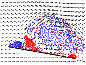
Figure 4. Flow field of a pitching and plunging plate at t/T = 0.25 and 0.40 for the case of α_eff,max = 24° from the traditional discrete vortex method (a,b), improved discrete vortex method (c,d) and experimental measurement (e,f). The circles with dashed lines represent the LEV (yellow), wake (red) and secondary vortex (SV; green).

Figure 5. Streamlines of a pitching and plunging plate at t/T = 0.25 and 0.40 for the case of α_eff,max = 24° from the traditional discrete vortex method (a,b), improved discrete vortex method (c,d) and experimental measurement (e,f).

The introduction of the secondary vortex in the improved method obviously changes the evolution of the flow topology (middle column in figures 4 and 5). With the development of the LEV, an increasing number of positive free vortices appear above the plate and move into the flow field. Some positive free vortices are dispersed in the range of the LEV. The other free vortices fill in the empty space under the leading-edge shear layer and constitute the secondary vortex. The boundary of the LEV is deformed under the influence of the secondary vortex at t/T = 0.25. With plate motion, more positive free vortices flow into the secondary vortex. The development of the secondary vortex cuts off the connection between the LEV and the feeding shear layer. Without the vorticity supply through the leading-edge shear layer, the LEV cannot maintain a stable structure. Different from that, the LEV reaches the trailing edge with stable vortex structure in the traditional method. To verify the accuracy of the improved discrete vortex method, the vorticity field with velocity vectors and streamlines from experimental measurements are also shown in figures 4 and 5 (right column), respectively. Compared with the traditional method (left-hand column in figures 4 and 5), the improved method better simulates the evolution of flow field, especially the detachment of the LEV. The similar distribution of singular point between the improved method and experiment also indicates that the improved method is superior to the traditional method.

Although the improved discrete vortex method better reconstructs the LEV detachment, the flow field remains slightly different from the flow of the experiment. The radii of the LEV and the secondary vortex in the experiment are smaller than those in the improved method, especially at t/T = 0.40. The leading-edge shear layer is preserved in the experiment measurement. The meeting between the large secondary vortex and the leading-edge shear layer in the improved method leads to the absence of rotational streamline. The three-dimensional instability of the LEV during convection in the experiment is one other main reason for the difference. Ol et al. (2009) found that the three-dimensional deformation of the LEV was unavoidable even without obvious wingtip spanwise flow. Both Rosti, Omidyeganeh & Pinelli (2016) and Guillaud, Balarac & Goncalvès (2018) found that the spanwise flow due to the three-dimensional deformation of the LEV was important. As suggested by the vorticity transport theorem (Akkala & Buchholz 2017), the spanwise flow reduces the radius of the LEV in the cross-section plane, which changes the covering range of the LEV in the developed phase. In addition, the interaction between the secondary structure and the LEV is strong viscous flow. The linear reconstruction of the flow field by the discrete vortex method ignores the nonlinear velocity fluctuation due to the viscous effect. The viscous effect on the development of vortex structure accelerates the dissipation of secondary vortex. This leads to the increase of vortex area in the discrete vortex method. The increase of secondary vortex size cuts off the connection between the LEV and the feeding shear layer in the discrete vortex method.

Furthermore, the lift coefficient variations for the different methods are calculated and shown in figure 6. The definition of lift coefficient in the experiment is ${C_L} = L/0.5\rho cbU_\infty ^2$. Here b is the span of the plate model. The formation of a secondary vortex in the improved method leads to an earlier decrease in lift coefficient than the traditional method. The descending rate of the lift coefficient in the improved method is much closer to the lift variation in the experiment. Thus, the improved method has better performance in the simulation of detachment of the LEV and the decrease of overall lift. Because both the trailing-edge angle and thickness of the plate force the wake to deviate from the chord line of the plate, there is a slight offset between experiment and the discrete vortex method. The difference between the discrete vortex method and experiment in flow field is another reason for the offset in lift coefficient. The deviation between the calculated lift of the discrete vortex method and the actual lift was also found in other studies, such as Xia & Mohseni (2013) and Li & Wu (2016). It suggests that the deviation is a common phenomenon in the discrete vortex method. Thus, the improved method can reconstruct the flow and calculate the aerodynamic force of the pitching and plunging plate.

Figure 6. Lift coefficient variation for the case α_{eff ,max} = 24° from different methods.

4.2. Interaction between secondary vortex and LEV

Based on the improved discrete vortex method, the interaction between the secondary vortex and the LEV is studied. Figure 7 shows the velocity field and distribution of the point vortices from the traditional and improved discrete vortex methods in different time periods. In comparison, the traditional method helps show the evolution of the LEV without the influence of a secondary vortex. At the beginning of plate motion, the negative point vortices that formed at the leading edge gather together and constitute the LEV. For the improved method, the positive point vortices that formed at the plate surface are spread among the LEV. Figure 8 further shows the streamlines from the traditional and improved discrete vortex methods. The similar LEV evolutions in the two methods indicate that the dispersed positive point vortices have a negligible effect on the LEV in the early LEV growth stage. The accumulation of positive point vortices at the leading edge forms the secondary vortex and gradually changes the evolution of the LEV. With the plate motion, more and more positive point vortices start to gather together instead of flowing into the LEV.

Figure 7. Velocity fields and point vortex distributions of the improved (a,c,e,g) and traditional (b,d,f,h) discrete vortex methods in different time periods for the case α_{eff ,max} = 24°.

Figure 8. Streamlines of the improved (a,c,e,g) and traditional (b,d,f,h) discrete vortex methods in different time periods for the case α_{eff ,max} = 24°.

In order to study how the point vortices accumulate upstream of the LEV and form the secondary vortex, the near-wall tangential velocity (u_s) along the vorticity layer is calculated and shown in figure 9. The negative velocity is the reverse flow brought by the LEV, and the positive velocity near the leading edge represents the development of secondary vortex. The isolines of u_s/U_∞ = −0.5 are also plotted in the figure to better show the development of vortex structure. At the beginning of plate motion, the near-wall tangential velocity distributions between the two methods are similar, which indicates that the positive vortices cannot change the development of the LEV at this stage. With the downstream movement of the LEV, the tangential velocity distribution near the leading edge is different. A low-speed area ahead of the recirculation zone is distinguished in the traditional method, due to the increasing gap between the LEV and feeding shear layer. The growing size of the LEV is the main reason for the low-speed area. The secondary vortex fills the space in the improved method. It is assumed that the low-speed area slows down the positive point vortices in the improved method, which leads to the accumulation of point vortices. These merged point vortices attract more point vortices and form the secondary vortex. Thus, the low-speed area because of the movement of the LEV is necessary for the formation of the secondary vortex.

Figure 9. The near-wall tangential velocity from (a) improved method and (b) traditional method for the case α_{eff ,max} = 24°. The solid line represents the isoline of u_s/U_∞ = −0.5 in the corresponding methods.

Besides, the near-wall tangential velocity distribution also shows that the secondary vortex remains motionless until the time of t/T = 0.35. In order to further study the effect of secondary vortex on the LEV, the shear layer angle is calculated and shown in figure 10. Because the growth of the LEV relies on the feeding vorticity through the leading-edge shear layer, the shear layer angle helps to reveal the development of the LEV. Here, the shear layer angle is assumed to be the angle between the plate and the fitting line of numerous newly generated point vortices at the leading edge. Because the positive point vortices near the leading edge influence the distribution of negative point vortices, small-scale fluctuations are obvious for the improved method. The localized regression method is used to better show the variation trend.

Figure 10. Change in leading-edge shear layer angle from the (a) improved method and (b) traditional method for the case α_{eff ,max} = 24°.

For the traditional method, the shear layer angle is highly dependent on the variation of the effective angle of attack. The effective incoming flow condition determines the development of the LEV. Different from that, an obvious plateau is found for the improved method in the time of 0.15 < t/T < 0.32, when the secondary vortex forms and grows in size. In the experimental studies of Li et al. (2020) and Kissing et al. (2020a), the plateau of shear layer angle represents the time when the secondary vortex starts to influence the development of the LEV. They suggested that the secondary vortex made the LEV accelerate moving downstream. The result in this research further verifies that the growth of secondary vortex is the dominant reason for the quasi-steady variation. Besides, the decrease of shear layer angle happens at the same time when the secondary vortex starts to move downstream. This indicates that the growing secondary vortex cuts off the connection between the LEV and feeding shear layer. The induced velocity of secondary vortex leads to the decrease of shear layer angle. Thus, the development of secondary vortex can be concluded as three stages. First, the existence of a low-speed area due to the growing LEV helps the formation of secondary vortex. Then, the secondary vortex grows in size and squeezes the LEV. Lastly, the developed secondary vortex moves downstream and leads to the detachment of the LEV.

4.3. The LEV lift generation mechanism

In the discrete vortex method, the flow structure is constituted by the point vortices which formed in the same position. For instance, the rotational flow of the LEV is assumed to be constituted by all point vortices formed at the leading edge. Depending on the lift calculation method, which is based on the vortical impulse formula (Wu 1981; Li & Lu 2012), the overall lift can be decomposed into lift contributions from different flow structures:

(4.1)\begin{equation}\left. {\begin{array}{*{20}{l@{}}} {\dfrac{L}{\rho } = \dfrac{\textrm{d}}{{\textrm{d}t}}\left( {\sum {{\varTheta_b}} + \sum {{\varTheta_{LEV}}} + \sum {{\varTheta_{wake}}} + \sum {{\varTheta_{SV}}} } \right),}\\ {{\varTheta_{()}} = {x_{()}}{\varGamma_{()}}.} \end{array}} \right\}\end{equation}

Here, $\varTheta$₍₎ is the vertical part of the vorticity moment of each point vortex, x ₍₎ is the horizonal location of the point vortex in the body frame and $\varGamma$₍₎ is the point vortex strength. The subscripts represent the flow structure, where b indicates the bound vortex on the plate, LEV indicates the LEV, wake indicates the wake and SV indicates the secondary vortex. The lift contribution from the newly introduced secondary vortex is also extracted from this. Figure 11 shows the lift contribution from different flow structures based on equation (4.1). The LEV has a mostly negative effect on the overall lift according to the applied lift calculation method here. Different from that, the lift contributions from other flow structures remain mainly positive. Among them, the lift contribution of secondary vortex in the LEV growth stage is small due to the weak vortex strength and low induced velocity. As the positive vortices accumulate and form a concentrated vortical structure, the induced velocity at each point vortex rapidly increases. The lift contribution of positive point vortices rapidly increases due to the formation of the secondary vortex.

Figure 11. Overall lift variation (blue line) and lift contribution from different assemblies of point vortices in the improved discrete vortex method for the case α_{eff ,max} = 24°.

To study the reason for the production of lift from different flow structures, figure 12 shows the lift coefficient contribution of each free vortex at t/T = 0.40. Because the lift contribution of the flow structure is based on the generating lift of contained point vortices, the production of lift of each point vortex helps study the lift mechanism of the flow structure. For any single free vortex in the flow field, because its circulation remains constant after generation, its lift contribution is expressed as

(4.2)\begin{equation}{L_v} = \rho {\varGamma _v}{u_v}.\end{equation}

Both magnitude and direction of the free vortex velocity determine its lift contribution. The opposite velocity directions at the upper side and bottom of the LEV result in opposite lift contributions. In addition, the velocity on the upper side of the LEV is higher than that on the bottom, which makes the overall lift contribution of the LEV negative.

Figure 12. Lift coefficient contribution of point vortex in (a) the LEV and wake and (b) secondary vortex at the time of t/T = 0.40 for the case α_{eff ,max} = 24°.

The decreasing lift contribution of the LEV is also found in the studies of starting plate through the discrete vortex method (Li & Wu 2015, 2016). They found that the increase of distance between the vortex and the plate led to a decrease of lift. However, it is found that the negative pressure peak keeps increasing at the beginning of plate motion with the formation of LEV (Feng, Li & Chen 2020). This indicates that the LEV may make a contribution to the increase of lift during its formation stage. Thus, the classical force decomposition based on flow structures cannot completely represent the vortex lift. It is necessary to find another way to estimate the vortex lift to better study the lift generation mechanism of the LEV.

To solve this problem, a further force decomposition method based on the decomposition on the circulation of bound vortex and the velocity of free vortex is proposed here. The vortex lift of vortex structure is extracted through the proposed force decomposition method in this research. According to the position of the point vortex, it can be divided into the free vortex which can move in the flow field and the bound vortex which is fixed on the plate. Different from the free vortex, the bound vortex fixed on the plate is not directly relevant to the flow structure. As the classical thin airfoil theory states, the bound vortex fixed on the plate is introduced to satisfy the boundary condition on the plate. The circulation of the bound vortex is determined by the induced velocity distribution on the plate. Thus, it can be decomposed into two parts depending on the external disturbance source:

(4.3)\begin{equation}{\varGamma _b} = {\varGamma _{b,p}} + {\varGamma _{b,v}}.\end{equation}

Here, $\varGamma$_b,p and $\varGamma$_b,v are the bound vortex distributions due to the influence of plate motion and free vortices, respectively. A similar decomposition on the bound vortex is also used by Xia & Mohseni (2013) and Li & Wu (2016). Then, the lift contribution of the bound vortex can be decomposed based on the external disturbance source (equation (4.3)) as

(4.4) \begin{align} \dfrac{{{L_b}}}{\rho } & = \dfrac{\textrm{d}}{{\textrm{d}t}}\left( {\sum {{x_b}{\varGamma_b}} } \right)\notag\\ & = \underbrace{{\sum {{x_b}\left( {\dfrac{\textrm{d}}{{\textrm{d}t}}{\varGamma_{b,p}}} \right)} }}_{{\textit{Added}\;\textit{mass}}} + \sum {{x_b}\left( {\dfrac{\textrm{d}}{{\textrm{d}t}}{\varGamma_{b,LEV}}} \right)} + \sum {{x_b}\left( {\dfrac{\textrm{d}}{{\textrm{d}t}}{\varGamma_{b,wake}}} \right)} + \sum {{x_b}\left( {\dfrac{\textrm{d}}{{\textrm{d}t}}{\varGamma_{b,SV}}} \right)} . \end{align}

Here, the subscript b refers to the bound vortex. The added mass represents the lift contribution from surrounding fluid acceleration due to plate motion. The other parts can be assumed as the lift contribution of corresponding flow structures.

For the free point vortex, as equation (4.2) states, its lift contribution is mainly determined by the motion velocity. The different sources of velocity represent the different kinds of lift contribution. For the case of a point vortex above a wall, the generating lift of the point vortex is positive due to its induced velocity. However, in the case with strong positive free-stream velocity, the motion direction of the point vortex is changed. The production of lift of the point vortex is determined by the free-stream velocity, which leads to confused lift contribution results. Thus, the vortex lift is supposed to be the generating lift of the point vortex in the vortex-dominated flow. Decomposition to the velocity field is needed to get the variation of vortex lift.

In the discrete vortex method, the velocity field is a combination of the translation velocity of the plate and the induced velocity of every point vortex. Thus, the decomposition approach to bound vortex can also be applied to the velocity field. Based on that, the velocity field can be written as U(u, v) = U_p + U_m. Here, U_p is the velocity field due to the plate motion and the bound vortex and U_m is the velocity field due to the free vortex. Velocity fields U_p and U_m are calculated by

(4.5)\begin{equation}\left. {\begin{array}{*{20}{c@{}}} {{\boldsymbol{U}_p} = {\boldsymbol{U}_t} + \boldsymbol{U}({\varGamma_{b,p}}),}\\ {{\boldsymbol{U}_m} = \boldsymbol{U}({\varGamma_{b,v}}) + \boldsymbol{U}({\varGamma_v}).} \end{array}} \right\}\end{equation}

Here, U_t is the relative translation velocity of the plate, U($\varGamma$_b,p) and U($\varGamma$_b,v) are the induced velocities of different parts of the bound vortex and U($\varGamma$_v) is the induced velocity of the free vortex. Through the calculation, U_p is independent of the vortex structures in the flow field, since $\varGamma$_b,p is only determined by the plate motion. Thus, U_p can be called the quasi-potential flow, which represents the flow field without flow separation due to plate motion. Correspondingly, U_m can be called the vortex-induced flow because it is determined by the distribution of the free vortex. The generated point vortices at the leading edge move with quasi-potential flow and form the shear flow. The production of lift of point vortices in quasi-potential flow cannot be assumed as the vortex lift. In contrast, the vortex-induced flow comes from the induced velocity of surrounding point vortices, which is the source of vortex-induced flow.

The decomposition to the velocity field is inspired by the classical Helmholtz–Hodge decomposition, which decomposes the velocity field into potential and solenoidal parts (Wu et al. 2007b). Here, the quasi-potential flow and the vortex-induced flow are analogous to the potential part and the solenoidal part, respectively. However, the point vortex model in this research satisfies the potential flow condition except for the vortex centre area. Thus, most of the vortex-induced flow is still irrotational, and the flow near the plate surface in quasi-potential flow cannot satisfy the potential flow condition. It cannot be concluded that the decomposition of the velocity field is equal to the Helmholtz–Hodge decomposition.

Figure 13(a–c) shows the decomposition of the velocity field at the time of t/T = 0.25, including the original flow (U), quasi-potential flow (U_p) and vortex-induced flow (U_m). The free vortices in the flow field and the corresponding bound vortex constitute the vortex-induced flow. In the vortex-induced flow field, the free vortices on the suction side of the plate constitute the rotational flow of the LEV. The velocity distribution in the LEV is not of central symmetry. The velocity at the bottom of the LEV is much higher than that on the upper side. The difference in velocity magnitude indicates that the induced velocity of the negative vortex above the plate points upstream. The line-like distribution of the point vortex in the wake has a limited influence on the vortex-induced flow. Because the free vortices that constitute the secondary vortex also contribute to the vortex-induced flow in the suction side of the plate, figure 13(d) shows the LEV-induced flow, which only calculates the induced velocity of negative free vortices in the LEV. The rotational flow in vortex-induced flow is similar to the LEV-induced flow. However, the velocity magnitude of the rotational flow in the LEV-induced flow is larger. Thus, the secondary vortex has a limited effect on the LEV structure before it grows. The growth of the secondary vortex can weaken the LEV strength.

Figure 13. Magnitude of the streamwise velocity with velocity vectors at t/T = 0.25 in the (a) original flow, (b) quasi-potential flow, (c) vortex-induced flow and (d) LEV-induced flow for the case α_{eff ,max} = 24°.

The decomposition on the velocity field can be applied to the lift calculation method. Since the circulation of free vortices remains constant after generation, the lift contribution of free vortices is decomposed according to the velocity field:

(4.6)\begin{equation}\frac{{{L_v}}}{\rho } = \frac{\textrm{d}}{{\textrm{d}t}}\left( {\sum {{x_v}{\varGamma_v}} } \right) = \sum {{\varGamma _v}\left( {\frac{\textrm{d}}{{\textrm{d}t}}{x_v}} \right) = } \sum {{\varGamma _v}{u_{v,p}}} + \sum {{\varGamma _v}{u_{v,m}}} .\end{equation}

Here, the subscript v refers to the free point vortices that constitute the LEV, wake and secondary vortex, subscript p refers to the velocity in the quasi-potential flow part and subscript m refers to the velocity in the vortex-induced flow part. The number of free vortices increases in every time step due to the generation of a point vortex. Li & Wu (2015) stated that the lift contribution of a new generating point vortex had limited influence on the overall lift. In this research, it is found that the lift contribution of generating point vortex in leading edge and trailing edge remain constant during plate motion. The corresponding part is neglected here.

Then, the overall lift can be rewritten as

(4.7) \begin{equation} \frac{L}{\rho } = \underbrace{{\sum {{x_b}\left( {\frac{\textrm{d}}{{\textrm{d}t}}{\varGamma_{b,p}}} \right)} }}_{{\textit{Added}\;\textit{mass}}} + \underbrace{{\sum {{\varGamma _v}{u_{v,p}}} }}_{{\textit{Fundamental}\;\textit{lift}}} + \underbrace{{\sum {{x_b}\left( {\frac{\textrm{d}}{{\textrm{d}t}}{\varGamma_{b,v}}} \right)} + \sum {{\varGamma _v}{u_{v,m}}} }}_{{\textit{Vortex}\;\textit{lift}}}.\end{equation}

The added mass is unrelated to the flow structure in the flow field. Thus, the other two parts, fundamental lift and vortex lift, represent the lift contribution of the flow structure. The fundamental lift represents the lift contribution due to the movement of point vortex in quasi-potential flow, and the vortex lift part represents the lift contribution in vortex-induced flow. Then, the lift coefficient contribution of the LEV and wake can be written as

(4.8) \begin{align}\left. {\begin{array}{*{20}{c@{}}} {{C_{L,LEV}} = \dfrac{1}{{0.5U_\infty^2c}}\Bigg[ {\underbrace{{\sum {{\varGamma_{LEV}}{u_{LEV,p}}} }}_{{\textit{Fundamental}\;\textit{lift}}} + \underbrace{{\sum {{x_b}\left( {\dfrac{\textrm{d}}{{\textrm{d}t}}{\varGamma_{b,LEV}}} \right)} + \sum {{\varGamma_{LEV}}{u_{LEV,m}}} }}_{{\textit{Vortex}\;\textit{lift}}}} \Bigg],}\\ {{C_{L,wake}} = \dfrac{1}{{0.5U_\infty^2c}}\Bigg[ {\underbrace{{\sum {{\varGamma_{wake}}{u_{wake,p}}} }}_{{\textit{Fundamental}\;\textit{lift}}} + \underbrace{{\sum {{x_b}\left( {\dfrac{\textrm{d}}{{\textrm{d}t}}{\varGamma_{b,wake}}} \right)} + \sum {{\varGamma_{wake}}{u_{wake,m}}} }}_{{\textit{Vortex}\;\textit{lift}}}} \Bigg].} \end{array}} \right\}\end{align}

Figure 14 shows the lift contribution of the LEV and wake in quasi-potential flow and vortex-induced flow. For the lift contribution of the LEV, the streamwise velocity in the quasi-potential flow keeps the corresponding lift contribution negative. With the development of the LEV, the reverse flow in the bottom of the LEV in the vortex-induced flow produces a positive lift contribution, which decreases the negative lift contribution brought about by the quasi-potential flow. For free vortices in the wake, the consistent streamwise velocity in quasi-potential flow makes a steadily rising lift contribution. After the formation of TEV, the lift contribution from the free vortices of the wake in vortex-induced flow starts to significantly decrease, due to the induced velocity of the LEV.

Figure 14. The variation of fundamental lift and vortex lift of (a) the LEV and (b) wake for the case α_{eff ,max} = 24°.

The above discussion indicates that the lift generation mechanism of the LEV is complex. Both the positive lift contribution in a vortex-induced flow and the negative lift contribution in a quasi-potential flow are parts of the lift contribution of the LEV. Because the velocity field in the quasi-potential flow is determined by the plate motion, the corresponding lift force is independent of the LEV development. Conversely, the lift contribution in the vortex-induced flow relies on the growth of the vortex structure. After the formation of the LEV, a reverse flow is found above the plate. The reverse flow in the vortex-induced flow generates lift. With the growth of the LEV, the reverse flow becomes stronger and generates higher lift. Thus, the vortex lift of the LEV can be defined as the lift force of the LEV in vortex-induced flow. The vortex-induced flow field is necessary to obtain the change in vortex lift of the LEV.

It should be noted that the chosen Reynolds number is in the range of O(10⁵). According to Ashraf, Young & Lai (2011) and Baik et al. (2012), an increase in Reynolds number weakens the LEV strength. Furthermore, the low vertical leading-edge velocity due to low Strouhal number and reduced frequency limits the increase in LEV strength (Li et al. 2020). Thus, the positive lift force generated by the LEV is not prominent in this study. In the other cases, like low Reynolds numbers and high Strouhal numbers, a positive lift contribution is also expected.

The interaction between secondary vortex and LEV, and the subsequent lift variation are concluded as shown in figure 15. The top-left panel, which shows the changes in overall lift and vortex lift, reveals the contribution of the vortex lift to the overall lift. The vortex lift continues to increase after the overall lift reaches its maximum. The increase in vortex lift helps maintain the slow decline in overall lift. When the vortex lift starts to decrease, the overall lift rapidly decreases. Thus, the proposed force decomposition method solves the contradiction about the negative lift contribution of the LEV with vortical-impulse theory in the discrete vortex method. Furthermore, the development of the flow structure in different time periods is shown in the top-right panel. The blue and red lines are the boundary of LEV and secondary vortex according to the accumulation of point vortices, respectively. Based on that, the lift generation mechanism is able to be revealed. The LEV grows at the beginning of plate motion, followed by an increase in the vortex lift and overall lift. With the development of the LEV, the growing secondary vortex is found below the LEV. In this stage, the secondary vortex has a limited influence on the LEV, and the vortex lift keeps increasing at this stage. When the secondary vortex grows larger, the connection between shear layer and LEV is weakened. As the secondary vortex cuts off the shear layer, the leading-edge shear layer drops to the plate surface without the support of the LEV. The loss of vorticity transport in the shear layer leads to an unstable vortex and corresponding decline of vortex lift. The chordwise movement of secondary vortex pushes the LEV and leads to the final the detachment of the LEV. The interruption from the secondary vortex to the leading-edge shear layer and LEV limits the increase in vortex lift. The detachment of the LEV decreases the vortex lift and follows a rapid decrease in overall lift.

Figure 15. Vortex lift of LEV and boundary of vortex structures during plate motion in the improved discrete vortex method.

Thus, the estimation of vortex lift in this research provides a new insight into the lift generation mechanism of the LEV. It indicates that the calculated force from vortical impulse method cannot represent the lift contribution of vortex structure. The confusion about the decrease of LEV generating lift is resolved through the decomposition on the velocity field and lift variation.

4.4. Vortex lift indicator based on the flow field in viscous flow

In the discussion above, both the lift generation mechanism of the LEV and the interaction between vortex structures are studied based on the inviscid flow of the improved discrete vortex method. The application of these findings in actual viscous flow needs further verification. Based on that, the estimation on the LEV generating lift is needed to study the variation of vortex lift. However, the force decomposition is not easy to accomplish in experiment measurement, especially the part of velocity decomposition. An easy and robust vortex lift indicator is needed to estimate the variation of vortex lift during plate motion.

According to the proposed lift generation mechanism of the LEV, the vortex-induced flow is essential for the calculation of vortex lift. Because the reverse flow on the suction side of the plate can be found only after the formation of the LEV, the reverse flow is assumed to be the characteristic flow in the vortex-induced flow of the LEV. Thus, the reverse flow strength is assumed to correspond to the LEV strength in a vortex-induced flow. In addition, the reverse flow is connected with the low-pressure zone on the suction side, which is assumed to be the effect of the lift contribution of the LEV (Feng et al. 2020; Kissing et al. 2020b; Li & Feng 2022). In the discrete vortex method, the unsteady Bernoulli theorem is also used to calculate the surface pressure (Ramesh et al. 2014). The calculation method is

(4.9)\begin{equation}{p_s}(x) = \rho \left( { - \frac{1}{2}u_s^2(x) - \frac{{\partial {\boldsymbol{\varPhi}_s}(x)}}{{\partial t}}} \right).\end{equation}

Here, $\boldsymbol{\varPhi}$_s is the surface velocity potential. In the inviscid numerical simulation of the starting plate at a large angle of attack, Li & Wu (2016) found that the steady part $( - u_s^2(x)/2)$ contributed most to the pressure distribution, especially the low-pressure zone under the LEV. Thus, the reverse flow strength can be used to reflect the suction force of the low-pressure zone and vortex lift of the LEV.

In order to estimate the reverse flow strength of the LEV, the Lamb vector (l ≡ ω × U) in the vertical direction is introduced in this research as the vortex lift indicator. The integral of the Lamb vector, which is closely related to the vortical impulse method, is also a classical method for the estimation of overall aerodynamic force (Marongiu & Tognaccini 2010; Wang et al. 2013). An indicator based on the Lamb vector, not vorticity or velocity magnitude, is more physical in the representation of the reverse flow strength and generating lift of vortex structure.

Because this research focuses on the lift variation and generation mechanism, only the value of the Lamb vector in the vertical direction is calculated here. Figure 16(a) shows the distribution of the non-dimensional value of the vertical Lamb vector $(c\omega_z u/U_\infty ^2)$ in the experimental case of α_eff,max = 24° in different time periods. With the development of the LEV, the reverse flow becomes obvious and leads to a higher value of the vertical Lamb vector. This means that the value of the vertical Lamb vector is able to represent the variation of reverse flow strength. According to that, the non-dimensional maximum value of the vertical Lamb vector $(l_{max}^\ast= c{(\omega_z u)_{max}}/U_\infty ^2)$ in the flow field is adopted as the vortex lift indicator of the LEV. In order to exclude the influence of wake and secondary vortex, only the region of negative vorticity is considered. The variations of vortex lift indicator and overall lift coefficient are shown in figure 16(b). The variations of vortex lift indicator and overall lift are quite similar, which means that the vortex lift indicator has good performance in the estimation of maximum overall lift.

Figure 16. (a) The distribution of non-dimensional vertical Lamb vector value $(c\omega_z u/U_\infty ^2)$ in different time periods for the experimental case α_{eff ,max} = 24°. The yellow diamond represents the location corresponding to the maximum vertical Lamb vector value. The corresponding value is assumed as the vortex lift indicator, and the location is called the vortex lift indicator location. (b) The variation of overall lift coefficient and the vortex lift indicator. The vertical dashed lines represent the time periods in the distribution of non-dimensional vertical Lamb vector value.

To further verify the practicality of the proposed indicator in more experimental cases, figure 17 shows the changes in overall lift and vortex lift indicator in the cases of different maximum effective angles of attack. The vortex lift indicator and overall lift reach a maximum simultaneously in all tested cases. The increase of vortex lift indicator with maximum effective angle of attack is consistent with the variation of maximum overall lift. Besides, all curves of the vortex lift indicator exhibit a similar development, and accordingly, three phases can be identified. These three phases are demarcated in figure 17 using a grey background. In the first phase, the indicator remains below zero. The lift from the quasi-potential flow is the main reason for the increase in overall lift. With the development of the LEV, a stronger reverse flow generates higher vortex lift in the second phase. The vortex lift of the LEV is the main source of the overall lift in the increasing phase. In the third phase, the vortex lift rapidly decreases because of the detachment of the LEV. This means that the proposed vortex lift indicator can be used to estimate the time and magnitude of the maximum lift.

Figure 17. Lift coefficient and proposed vortex lift indicator in the cases of (a–d) different maximum effective angles of attack in experimental measurements. The different grey backgrounds represent the development phases of vortex lift indicator.

Based on the proposed vortex lift indicator, the lift generation mechanism of LEV in actual viscous flow is examined. Figure 18(a) shows a schematic diagram of the positions of vortex centre and vortex lift indicator. Because the vortex lift indicator represents the strength of strongest reverse flow in the LEV, the vortex lift indicator is assumed to be located in the vortex core boundary. The vortex core is the part of the vortex with strong rotational flow, which contributes most to the production of lift of the LEV. Based on that, the connection between vortex evolution and producing lift is able to be better studied. Figure 18(b) shows the locations of vortex lift indicator and vortex centre of the LEV in the reference frame of plate in the case of α_eff,max = 32°. The vortex centre is determined based on $\varGamma$₁ criterion (Graftieaux, Michard & Grosjean 2001). Considering the seemingly linear movement of vortex centre and vortex lift indicator, the fitting line is used to show the trajectories of vortex centre and vortex lift indicator. Figure 18(c–e) shows the fitting line of vortex centre and vortex lift indicator for the cases of α_eff,max = 24°–40°. The red and orange lines represent the vortex lift indicator in increasing and decreasing phase, respectively. The vertical distance between the vortex centre and vortex lift indicator is calculated and shown in figure 18(f). The calculated vertical distance represents the radius of vortex core to some extent. Among all the tested cases, the area of vortex varies little during the vortex lift increasing phase. For the cases of α_eff,max = 24° and 32°, the rapid increase of vortex core is connected with the decrease of vortex lift indicator. However, the area of vortex core varies slowly in the decreasing vortex lift phase for the case of α_eff,max = 40°. These results indicate that the lift generation mechanism of the LEV changes with an increase of α_eff,max.

Figure 18. (a) Schematic diagram of vortex core, vortex boundary, position of vortex centre and vortex lift indicator. (b) The distribution of vortex lift indicator (red symbols) and vortex centre (blue symbols) in the frame of the plate for the case α_eff,max = 32°. The blue line represents the fitting of vortex centre during its growth stage. The red and orange lines represent the vortex lift indicator in lift increasing phase and decreasing phase, respectively. (c–e) The movement trajectories of vortex lift indicator and vortex centre for the cases of α_eff,max = 24°, 32° and 40°. The vortex core is plotted according to the distance between vortex centre and vortex lift indicator. (f) The variation of the vertical distance between vortex lift indicator and vortex centre.

To study the development of LEV in different vortex lift phases, figure 19 shows the vorticity field and the locations of vortex centre and vortex lift indicator in experiments for the cases of α_eff,max = 32° and 40°. In the vortex lift increasing phase, the vortex structures in different cases are quite similar. The concentrated vorticity in the vortex core contributes to the increase of vortex lift. The vorticity input through the shear layer transfers into the growing vortex core and leads to an increasing vortex lift. Things change in the vortex lift decreasing phase. For the case of α_eff,max = 32°, the concentrated vorticity in vortex core cannot be found. The vortex strength of the LEV is gradually decreasing, which leads to a decline of vortex lift. Different from that, the vortex core remains stable in the decreasing vortex lift phase in the case of α_eff,max = 40°. However, the vorticity strength in the area outside of the vortex core is obviously smaller than that in the vortex centre. This indicates that the development of the vortex core is suppressed. A large α_eff,max gives sufficient space for the development of secondary vortex. The stronger interaction between secondary vortex and LEV limits the development of vortex core and leads to a decrease of vortex lift. Besides, the growing secondary vortex weakens the vorticity transport in the leading-edge shear layer. Without sufficient vorticity input, the size of vortex core shrinks while the vortex boundary is enlarged in later development.

Figure 19. The vorticity field, the location of vortex centre (black circle) and vortex lift indicator (red square) in the increasing (a,c) and decreasing (b,d,e) vortex lift phases.

Thus, the discussion above states that the proposed vortex lift indicator helps to study the lift enhancement mechanism of the LEV during dynamic stall. The accurate estimation of maximum lift and corresponding motion period means that the vortex lift indicator can be applied in other fields. In the research of an unsteady plate, the high inertia force makes it difficult to directly measure the aerodynamic force on the plate, especially in a wind tunnel. The proposed vortex lift indicator gives a new way to easily calculate the lift variation. Furthermore, a flapping wind turbine blade and other industrial applications can use this method to easily obtain the real-time lift variation.

5. Conclusion

This research gives an insight into the lift generation mechanism of the LEV of a pitching and plunging plate through the discrete vortex method and experiment. To obtain accurate LEV evolution, a formation condition of the secondary structure in the discrete vortex method is proposed to express the viscous effect between LEV and plate. The simulation of the secondary structure solves the shortcomings of the traditional discrete vortex method, which only focuses on the LEV and wake reconstruction. Compared with the experimental measurement results, the flow topology evolution and lift variation of the improved method are much closer to those of real flow. This means that the idea of introducing the secondary vortex gives a new way to model the viscous interaction between the vortex and surface, and not only in the case of evolution of LEV during dynamic stall. Based on that, the interaction between secondary structure and LEV is studied. The induced velocity is not the only parameter that determines the formation of the secondary structure. The low-speed area between the shear layer and the LEV is another necessary precondition for the secondary structure. With the development of secondary vortex, its growing size limits the development of the LEV. The chordwise movement of the secondary structure finally cuts off the leading-edge shear layer and leads to the detachment of the LEV.

In addition, the lift generation mechanism of the LEV is studied through the vortex evolution in the improved discrete vortex method. According to the induced velocity of the point vortex, the flow field can be decomposed into a quasi-potential flow and a vortex-induced flow. Here, the quasi-potential flow is the potential flow around the moving plate without flow separation, and the vortex-induced flow directly represents the vortical flow of concentrated vortex structure. The lift contribution of the vortex structure in vortex-induced flow can be assumed to be the vortex lift of the corresponding structure. The proposed definition of vortex lift helps to give a new way to solve the negative producing lift of the LEV with the application of vortical impulse theory. Based on the definition of vortex lift, the reversed flow of the LEV is also found to be a key feature that generates the positive lift contribution. The growth of the LEV enhances the reverse flow and increases the vortex lift. The high vortex lift supports the increase of overall lift and delays the decline in overall lift at a high angle of attack. Thus, a stable LEV with strong reverse flow in the flow field is important for high-amplitude lift at high angles of attack.

Consequently, a vortex lift indicator of the LEV that can be applied in experiments is further proposed. The maximum value of the vertical Lamb vector in the range of the LEV is used to estimate the generating lift of the LEV. The maximum overall lift and corresponding motion period are obtained accurately with the help of the proposed vortex lift indicator. Based on that, the lift generation mechanism of the LEV and the influence of secondary vortex are also verified in actual viscous flow. The vortex core which contributes mostly to the production of lift of the LEV is identified through the distance between vortex centre and vortex lift indicator. The unstable vortex core is the main reason for the decrease of lift in the case with small and medium maximum effective angles of attack. With the increase of maximum effective angle of attack, the dissipation effect from secondary vortex suppresses the growth of LEV and leads to a decrease of lift. Besides, the vortex lift indicator is a new way to easily obtain the lift variation from the velocity field. It gives a method to estimate the overall lift in wind tunnel experiments, flapping wind turbine blades and other similar industrial applications.