Exact solutions for steadily travelling water waves with submerged point vortices

Abstract

This paper presents a novel theoretical framework, based on the concept of the Schwarz function of a wave, for understanding water waves with vorticity in the absence of gravity and capillarity. The framework leads naturally to a taxonomy of three subcases, herein referred to as cases 1, 2 and 3, into which fall three existing studies of water waves incorporating uniform vorticity and submerged point vortices. This provides a theoretical unification of several seemingly unrelated results in the literature. It also provides a route to finding new exact solutions with this paper focussing on new solutions falling within the case 2 category. Among several presented here are a submerged point vortex pair cotravelling with a solitary deep-water wave, von Kármán point vortex streets cotravelling with a periodic deep-water wave and a point vortex row cotravelling with a wave in water of finite depth. Some other more exotic waveforms are also constructed. All these new solutions generalize those of Crowdy & Roenby (Fluid Dyn. Res., vol. 46, 2014) who found steady waves in deep water cotravelling with a submerged point vortex row for which the free surface shapes turn out to coincide with those of pure capillary waves on deep water found by Crapper (J. Fluid Mech., vol. 2, 1957). The new exact solutions are likely to provide a useful basis for asymptotic or numerical studies when additional effects such as gravity and capillarity are incorporated.

1. Introduction

The literature on two-dimensional water waves has historically focussed on irrotational flow in the presence of gravity or capillarity, or both, but there is growing interest in the theory of water waves with vorticity where finite-amplitude waves can exist even without either of these physical effects (Benjamin 1962; Simmen & Saffman 1985; Pullin & Grimshaw 1988; Teles da Silva & Peregrine 1988; Vanden-Broeck 1994, 1996; Sha & Vanden-Broeck 1995; Constantin & Strauss 2004; Groves & Wahlén 2007, 2008; Ehrnström 2008; Wahlén 2009; Hur & Dyachenko 2019a,b; Hur & Vanden-Broeck 2020; Hur & Wheeler 2020). A recent review article (Haziot et al. 2022) describes this history over the last two centuries and includes a survey of some of the literature on water waves with vorticity.

When introducing vorticity to steadily travelling water waves, one has a choice of the steady vorticity distribution and arguably the most common in the water-wave literature has been to take the vorticity to be uniform. Tsao (1959) performed an early weakly nonlinear analysis into this case. Using a weakly nonlinear formulation Benjamin (1962) found solitary wave solutions using a boundary integral formulation. Simmen & Saffman (1985) carried out a numerical study of this case for gravity waves in deep water; this was built upon later by Teles da Silva & Peregrine (1988) who studied the finite depth scenario. By now, much other numerical work has been done using a variety of formulations (Vanden-Broeck 1994, 1996; Sha & Vanden-Broeck 1995; Hur & Dyachenko 2019a,b; Hur & Vanden-Broeck 2020).

In the field of vortex dynamics a region of uniform vorticity is called a vortex patch (Saffman 1992). While this designation emerged from consideration of finite-area regions of uniform vorticity – an early classical example being the rotating Kirchhoff elliptical vortex patch (Saffman 1992; Lamb 1994) – the name now refers to any constant region vorticity, even one that is unbounded. Periodic travelling gravity waves with uniform vorticity might therefore be thought of as periodic vortex patches in steady unidirectional motion. Another popular vortex type is the hollow vortex model (Michell 1890; Pocklington 1895; Baker, Saffman & Sheffield 1976; Ardalan, Meiron & Pullin 1995; Crowdy & Green 2011; Telib & Zannetti 2011; Llewellyn Smith & Crowdy 2012; Crowdy, Llewellyn Smith & Freilich 2013). This model is arguably the radial geometry analogue of the irrotational water-wave problem, without gravity or capillarity, and where the free surface is now a closed curve: a hollow vortex is usually taken to be a finite-area, constant-pressure region with a free boundary having a non-zero circulation around it and typically surrounded by an otherwise irrotational flow. The main ingredients of the free boundary problem for a hollow vortex are therefore akin to those of irrotational water waves. Indeed, many mathematical techniques, such as free streamline theory, can be applied to both free boundary problems (Crowdy & Roenby 2014). The vortex patch and the hollow vortex are finite-area models of a vortex. Perhaps surprisingly, the simplest model of a vortex, namely, a point vortex with no spatial extent (Saffman 1992), has been used quite rarely in the water wave literature, although interest in it is increasing. Early work on the rigorous existence theory, when gravity is present but weak, and when the vorticity is modelled as a point vortex, was carried out by Filippov (1961) and Ter-Krikorov (1958). Shatah, Walsh & Cheng (2013) have proved the existence of steadily travelling two-dimensional capillary–gravity water waves with compactly supported vorticity, including the case where the vorticity is in the form of point vortices. Varholm (2016) has constructed solitary solutions for gravity–capillary waves with a submerged point vortex. Le (2019) looked at solitary waves carrying a submerged finite dipole in deep water, which is not unrelated to the point vortex problem if a point dipole is viewed as a limit of two point vortices of increasing equal and opposite circulation coalescing. It is a classical result that the equations of point vortex motion in free space have a Hamiltonian structure (Saffman 1992) and such a structure persists in the presence of a free surface. Rouhi & Wright (1993), who built on earlier work of Zakharov (1968), have shown that the equations for water waves with submerged point vortices is a Hamiltonian system.

Several analytical solutions are known for finite-amplitude travelling waves with vorticity without gravity or surface tension. Crowdy & Nelson (2010) found a class of exact solutions to the problem of travelling waves on a deep-water linear shear current having constant vorticity and with an additional submerged cotravelling point vortex row. The techniques used to construct those solutions were borrowed from an earlier study of Crowdy (1999) who posed that streamfunctions taking the form of so-called modified Schwarz potentials can provide equilibrium vortical solutions of the Euler equations. Crowdy & Roenby (2014) derived an exact solution for finite-amplitude steadily travelling water waves, in the absence of gravity or surface tension, with a submerged freely cotravelling point vortex row in deep water and where the fluid is otherwise irrotational. Intriguingly, Crowdy & Roenby (2014) found that the free surface shapes in this problem are precisely those for irrotational pure capillary waves found by Crapper (1957). The results of Crowdy & Roenby (2014), where point vortices are freely convected with the surface wave, should be distinguished from other studies of point vortices interacting with free surfaces (Gurevich 1963; Shaw 1972; Forbes 1985; Doak & Vanden-Broeck 2017) where the point vortex is not free but is meant to serve as a mathematical model of an obstruction (Vanden-Broeck 2010) occluding flow in the fluid layer or jet flow near a solid surface. In the latter problems, a net external force keeps the vortex in place.

It has recently been discovered that Crapper's free surface profiles for pure capillary waves reappear, yet again, in the problem of water waves with constant vorticity but in the absence of gravity and surface tension (Hur & Wheeler 2020). Crowdy & Roenby (2014) had earlier attributed the surprising recurrence of Crapper's free surface shapes in a problem of vorticity-driven water waves to the fact that they have a more abstract mathematical significance as so-called double quadrature domains (Crowdy 2005, 2020), a point of view that is related mathematically to use of the Schwarz function of a curve (Davis 1974) to be advocated in the present paper.

This article has two main goals. The first is to present the novel framework, based on the Schwarz function of a wave, for understanding the problem of steadily translating water waves with vorticity when the vorticity distribution is taken to be uniform but including the possibility of additional submerged point vortices. This is done in § 2. The general framework naturally gives rise to a taxonomy comprising three special cases: they are designated here as cases 1, 2 and 3. This viewpoint turns out to provide a theoretical unification of the aforementioned work of Crowdy & Nelson (2010), Crowdy & Roenby (2014) and Hur & Wheeler (2020) which, respectively, are the most basic water-wave solutions falling within cases 1, 2 and 3. Beyond this unification, the framework also points to strategies for generating broader classes of new solutions. The focus here is on constructing new solutions falling within the case 2 categorization. Section 3 achieves the second goal of this paper which is to present a range of new exact solutions for point vortex configurations in otherwise irrotational flow freely cotravelling with steady waves on an interface. New solutions falling within cases 1 and 3 are also feasible, but this challenge will be tackled elsewhere.

2. Water waves and the Schwarz function

On a flat profile $y=0$ in a Cartesian $(x,y)$ plane, and using the complex variable ${z=x+{\rm i}y}$, it is trivial to say that

(2.1)\begin{equation} \bar{z} = z,\quad {\rm on}\ y=0. \end{equation}

An important observation, however, is that the right-hand side of (2.1) is an analytic function of $z$ that can be analytically continued off the line $y=0$. This function is a simple example of a Schwarz function (Davis 1974). Most commonly, these are defined for closed analytic curves, such as a circle or an ellipse for example. However, for a more general wave profile, $\partial D$ say, given by an analytic curve that is periodic in the $x$ direction, the Schwarz function of $\partial D$ can be defined as the function $S(z)$, analytic in a strip containing the wave profile, satisfying the conditions

(2.2)\begin{equation} S(z) = \bar{z},\quad {\rm on}\ \partial D, \end{equation}

with

(2.3)\begin{equation} S(z) \to z + {\rm i} \lambda + {O}(1/z),\quad {\rm as}\ y \to -\infty,\quad \lambda \in \mathbb{R}. \end{equation}

From (2.1) the Schwarz function for a flat profile $y=0$ is given identically by $S(z)=z$ and corresponds to $\lambda =0$. For more wavy periodic profiles, $S(z)$ is a more complicated function and (2.3) will only hold as $y \to -\infty$. Only wave profiles which are analytic curves can conveniently be described using the Schwarz function (Davis 1974) but this mild restriction is expected to include a wide range of steady water waves.

Indeed, consider the problem of steadily translating, periodic water waves with uniform vorticity $\omega _0$ in the semi-infinite region below the interface extending to $y \to -\infty$. Consideration here will include finite-depth fluid layers, which do not extend to $y \to -\infty$, and how to adapt the framework to such cases will be explained later. In a frame cotravelling with the spatially periodic waves the streamfunction $\psi$, from which the velocity is given by $\textbf{u} = (u,v) = ({\partial \psi /\partial y},\ -{\partial \psi /\partial x})$, satisfies

(2.4)\begin{equation} \nabla^2 \psi ={-} \omega_0. \end{equation}

On changing variables to $z=x+{\rm i}y$ and $\bar {z} = x-{\rm i}y$ we can write this as

(2.5)\begin{equation} 4\frac{\partial^2 \psi}{\partial \bar{z} \partial z} ={-}\omega_0 \end{equation}

which, on integration with respect to $\bar {z}$, yields

(2.6)\begin{equation} \frac{\partial \psi}{\partial z} ={-} \frac{\omega_0}{4} \bar{z} + \frac{C(z)}{2 {\rm i}}, \end{equation}

where $C(z)$ is an analytic function of $z$, which will be allowed to have possible simple pole singularities with purely imaginary residues in the flow region. Since (2.6) implies that

(2.7)\begin{equation} u - {\rm i} v = 2 {\rm i} \frac{\partial \psi}{\partial z} ={-} \frac{{\rm i} \omega_0}{2} \bar{z}+ C(z), \end{equation}

then if, near some point $z=z_a$ in the fluid, $C(z)$ has a Laurent expansion of the form

(2.8)\begin{equation} C(z) ={-} \frac{{\rm i} \varGamma}{2 {\rm \pi}(z-z_a)} + C_0 + C_1 (z-z_a) + \cdots,\quad \varGamma \in \mathbb{R}, \end{equation}

where $\lbrace C_j \in \mathbb {C} \,|\, j \ge 0 \rbrace$ are coefficients then, physically, the flow has a point vortex of circulation $\varGamma$ at $z_a$ (Saffman 1992). Such singularities are the only physically admissible ones of interest for this paper although other singularity types, such as point sources and dipoles, can, in principle, be considered within the framework developed here. On combining (2.7) and (2.8) the complex velocity field then has the local form near $z_a$ given by

(2.9)\begin{equation} u - {\rm i} v={-} \frac{{\rm i} \varGamma}{2 {\rm \pi}(z-z_a)} + X^{(z_a)}(z,\bar{z}), \end{equation}

where

(2.10)\begin{equation} X^{(z_a)}(z,\bar{z})={-} \frac{{\rm i} \omega_0}{2} \bar{z} + C_0 + C_1 (z-z_a) + \cdots . \end{equation}

It is crucial to note that for this point vortex to be in steady equilibrium we require that

(2.11)\begin{equation} X^{(z_a)}(z_a,\overline{z_a})=0. \end{equation}

This criterion is sometimes asserted to be a consequence of the Helmholtz laws of vortex motion but, since it represents a singular situation, Saffman (1992) invokes a more direct argument based on the condition that the vortex is free of net force.

A form of Bernoulli's theorem (Saffman 1992) carries over to two-dimensional incompressible flows with uniform vorticity and dictates that the fluid speed on an interface with a constant-pressure region must be constant, equal to $q$ say. Combined with the condition that the interface must be a streamline in the cotravelling frame it follows that

(2.12)\begin{equation} u + {\rm i}v = q \frac{{\rm d} z}{{\rm d} s},\quad z \in \partial D, \end{equation}

where ${\rm d} s=\sqrt {{{\rm d}x}^2+{{\rm d}y}^2}$ denotes the arclength element along $\partial D$ which we take to increase as $\partial D$ is traversed with the fluid region to the right (the opposite choice would simply reverse the sign of $q$). The complex conjugate of (2.12) combines with (2.7) to imply that, on the wave surface,

(2.13)\begin{equation} q \frac{{\rm d}\bar{z}}{{\rm d} s} ={-} \frac{{\rm i} \omega_0}{2} \bar{z}+ C(z),\quad z \in \partial D. \end{equation}

Writing this in terms of the Schwarz function (2.2) of $\partial D$ yields

(2.14)\begin{equation} q \sqrt{S'(z)} ={-} \frac{{\rm i} \omega_0}{2} S(z) + C(z),\quad {\rm or}\quad C(z) = q \sqrt{S'(z)} +\frac{{\rm i} \omega_0}{2} S(z),\quad z \in \partial D, \end{equation}

where we have used the fact that

(2.15)\begin{equation} \frac{{\rm d} \bar{z}}{{\rm d} s} = \sqrt{S'(z)},\quad z \in \partial D. \end{equation}

(Throughout this paper, the prime notation will be used to denote the derivative of a function with respect to its argument; in the case of a function of more than one variable, the derivative with respect to the first argument is assumed.) Equation (2.14) is now a relation between analytic functions that can be continued off the wave surface into the fluid region. From (2.7) the associated velocity field is then

(2.16)\begin{equation} u - {\rm i} v={-} \frac{{\rm i} \omega_0}{2} \bar{z}+ q \sqrt{S'(z)} + \frac{{\rm i} \omega_0}{2} S(z). \end{equation}

Condition (2.3) means that, as $y \to -\infty$,

(2.17)\begin{equation} u - {\rm i} v=\frac{{\rm i} \omega_0}{2} (z- \bar{z} + {\rm i} \lambda) + q ={-} {\omega_0 y} + \left (q- \frac{\lambda \omega_0}{2} \right ) \end{equation}

which corresponds to waves of speed

(2.18)\begin{equation} U = \frac{\lambda \omega_0}{2} - q \end{equation}

travelling on a semi-infinite simple shear with shear rate $-\omega _0$.

Since the general expression (2.16) for the conjugate velocity field depends on the two parameters $\omega _0$ and $q$, three natural cases, referred to as cases 1, 2 and 3 for the remainder of this paper, can now be distinguished.

2.1. Case 1: $q=0, \omega _0 \ne 0$

One choice is to set $q=0$ but to insist that $\omega _0 \ne 0$. Then, from (2.16), the complex velocity field becomes

(2.19)\begin{equation} u - {\rm i} v={-} \frac{{\rm i} \omega_0}{2} \left (\bar{z} - S(z) \right ). \end{equation}

Explicit solutions for waves on linear shear currents falling within this class have already been derived by Crowdy & Nelson (2010). In those solutions a single periodic vortex row in the lower fluid layer cotravels with a wave on the interface between air and a semi-infinite linear shear current in the lower half-plane. In this case the streamfunction takes the form of a so-called modified Schwarz potential (Crowdy 2005, 2020) and the idea that such functions might describe vortical equilibria of the two-dimensional Euler equation was first put forward by Crowdy (1999) in the context of finding equilibria for finite-area multipolar vortices comprising a vortex patch with a superposed distribution of point vortices. This general class of solutions, which we now call case 1, turns out to contain a wide variety of vortical equilibria of the Euler equations, many available in the form of exact analytical solutions (Crowdy 2002a,c; Crowdy & Marshall 2004, 2005). Because of these multifarious solutions in the ‘radial geometry’, many other solutions for water waves with vorticity generalizing those of Crowdy & Nelson (2010) are expected to exist within this class.

2.2. Case 2: $q \ne 0, \omega _0 =0$

A second choice is to set $\omega _0=0$ but to insist now that $q \ne 0$. In this case, there is no linear shear flow in the far field as $y \to -\infty$ and the flow is irrotational. From (2.16), the complex velocity field now becomes

(2.20)\begin{equation} u - {\rm i} v = q \sqrt{S'(z)}. \end{equation}

If the waveform is such that $\sqrt {S'(z)}$ has only suitable simple pole singularities in the fluid region, and also such that its integral $S(z)$ also has only simple pole singularities in the fluid region – this can clearly be expected to restrict the class of admissible waveforms considerably – then the flow will comprise a point vortex equilibrium, as will be shown in § 3 where this case is studied in more detail. A one-parameter family of explicit solutions within this class has been given by Crowdy & Roenby (2014). In those solutions a single periodic vortex row, with a single point vortex per period, cotravels with a wave on otherwise irrotational deep water. Intriguingly, the wave shapes found by Crowdy & Roenby (2014) coincide exactly with those for pure irrotational capillary waves on deep water as found by Crapper (1957). This circumstance is striking in view of the very different nature of the physical problem in each case.

The solution of Crowdy & Roenby (2014) appears to be the only solution within this class known in the previous literature. But it turns out that there are many other exact solutions falling with this case 2 scenario, and the objective of § 3 is to present a range of new solutions of this kind.

2.3. Case 3: $q \ne 0, \omega _0 \ne 0$

The remaining possibility is to allow $\omega _0 \ne 0$ and $q \ne 0$. In this case, (2.16) gives the velocity field which can be rewritten as

(2.21)\begin{equation} u - {\rm i} v ={-} \frac{{\rm i} \omega_0}{2} \bar{z}+ \frac{{\rm i} \omega_0}{2} \left ( S(z) - \frac{2{\rm i} q}{\omega_0} \sqrt{S'(z)} \right ). \end{equation}

If, as in case 2, the wave shape is chosen so that both $\sqrt {S'(z)}$ and $S(z)$ have a single simple pole singularity inside a typical period window of the fluid region, the bracketed term in (2.21) suggests it might be possible to pick the real parameter $q/\omega _0$ to remove this singularity in the complex velocity leaving a flow that is free of point vortices but still with uniform vorticity. As shown in detail in § 3, this is indeed possible, and the resulting solutions coincide with those found by Hur & Wheeler (2020), who used different methods, and who corroborated a series of earlier numerical computations (Hur & Dyachenko 2019a,b; Hur & Vanden-Broeck 2020) indicating that the free surface shapes in this case also coincide with the pure capillary waves of Crapper (1957).

It is already valuable that the above Schwarz function formulation, leading naturally to these three cases, provides a theoretical unification of the (until now apparently independent) previous water-wave studies of Crowdy & Nelson (2010), Crowdy & Roenby (2014) and Hur & Wheeler (2020). For example, with this understanding it is no longer surprising that the wave shapes found by Crowdy & Roenby (2014) and Hur & Wheeler (2020) are the same. This is discussed further in the next section. (It is still surprising, however, that the shared waveforms of Crowdy & Roenby (2014) and Hur & Wheeler (2020) happen also to be shared by the pure capillary waves of Crapper (1957).)

With the three cases set out, it is natural to ask if other solutions within each category can be found. Table 1 summarizes how published results already in the literature can now be understood within the case 1–3 taxonomy just described; both the periodic ‘water wave’ geometry and the radial ‘vortex’ geometry are surveyed in this table. Of particular note is that the ‘radial analogues’ of the case 3 water-wave solutions found by Hur & Wheeler (2020) have recently been identified by Crowdy, Nelson & Krishnamurthy (2021) and given the designation ‘H-states’ in analogy with the name ‘V-states’ given to rotating vortex patches. The table also indicates the many known solutions in the radial vortex geometry within the case 1 category and, as already mentioned, it is expected that analogous solutions exist in the water-wave geometry.

Table 1. Within the new case 1, 2 and 3 taxonomy, several existing analytical results in the literature, both in the periodic (water wave) and radial (vortex) geometries, can be understood within a unified theoretical framework.

The remainder of the present paper will focus on laying out new solutions, generalizing those already found by Crowdy & Roenby (2014), within the case 2 scenario. Further investigation of the case 1 and 3 scenarios is left for a future study.

3. Exploring case 2: point vortex equilibria with a free surface

In the cotravelling frame the complex velocity field for the case 2 situation is

(3.1)\begin{equation} u - {\rm i} v = q \sqrt{S'(z)}, \end{equation}

where $S(z)$ is the Schwarz function associated with the steadily translating wave profile satisfying (2.2) and (2.3). Suppose that, near some point $z_a$ in the fluid region, $\sqrt {S'(z)}$ has a simple pole with local expansion

(3.2)\begin{equation} \sqrt{S'(z)} = \frac{{\rm i} A}{z-z_a} + B + {O}(z-z_a),\quad A \in \mathbb{R}. \end{equation}

Consequently, according to (3.1), the local expansion of the complex velocity is

(3.3)\begin{equation} u - {\rm i} v = q \left (\frac{{\rm i} A}{z-z_a} + B + {O}(z-z_a) \right ). \end{equation}

It is seen now why $A$ is taken to be real since, physically, this corresponds to a point vortex at $z=z_a$ with circulation $-2 {\rm \pi}q A$. To satisfy the stationarity condition (2.11) it is clear that we require $B=0$. On squaring (3.2),

(3.4)\begin{equation} S'(z) ={-}\frac{A^2}{(z-z_a)^2} + \frac{2 AB {\rm i}}{z-z_a} + C + {O}(z-z_a), \end{equation}

where $C$ is some constant. Therefore, on integration, the local expansion of $S(z)$ is

(3.5)\begin{equation} S(z) = \frac{A^2}{z-z_a} + {2 AB}{\rm i} \log(z-z_a) + D + {O}(z-z_a), \end{equation}

where $D$ is an integration constant. The important observation is that if $B=0$, meaning that the point vortex is in equilibrium, then the Schwarz function will also have a simple pole at $z_a$ with no logarithmic singularity there. This imposes constraints on the functional form of $S(z)$ because a logarithmic singularity at $z_a$ must generally be expected at any point where $\sqrt {S'(z)}$ has a simple pole.

In summary, ensuring that there is a stationary point vortex at $z_a$ in the cotravelling frame is equivalent to finding a curve whose Schwarz function $S(z)$, as well as the square root of its derivative $\sqrt {S'(z)}$, has a simple pole at $z_a$. For a global steadily translating equilibrium, this must be true at any and all simple poles of $S(z)$ in the period window and, moreover, $S(z)$ must not have any other finite singularities in the fluid region. The function $S(z)$ always has a simple pole at infinity according to (2.3) but this is an inevitable consequence of seeking an $x$-periodic wave profile and, as stated earlier, is true even of the trivial flat profile $y=0$.

In view of these observations, the construction of travelling periodic, or solitary, waves on a free surface with submerged point vortices falling within this class can be carried out. Mathematically, the task is to find free surface profiles whose Schwarz function $S(z)$, as well as the square root of its derivative $\sqrt {S'(z)}$, have only simple poles in the fluid region. If a wave profile having these properties can be found then, by the considerations above, it automatically represents a steadily travelling wave with a submerged cotravelling point vortex distribution.

A convenient way to construct Schwarz functions with the requisite properties is to make use of conformal mapping from a canonical preimage domain in a parametric $\zeta$ domain. This was also done by Crowdy & Nelson (2010) in the case 1 scenario. To see why, consider a conformal mapping from the unit $\zeta$ disc, $|\zeta | <1$, given by

(3.6)\begin{equation} z = Z(\zeta) \end{equation}

to some fluid region of interest. The Schwarz function $S(z)$ can be written, as a function of $\zeta$, as

(3.7)\begin{equation} S(z) = \bar{z} = \overline{Z(\zeta)} = \overline{Z(1/\bar{\zeta})} = \bar{Z}(1/\zeta), \end{equation}

where we have used the fact that ${\zeta } =1/\bar {\zeta }$ on $|\zeta |=1$ and introduced the Schwarz conjugate function, $\bar {Z}(\zeta )$, of the analytic function $Z(\zeta )$ defined by $\bar {Z}(\zeta ) = \overline {Z(\bar {\zeta })}$. Moreover, it is easy to verify that

(3.8)\begin{equation} \sqrt{S'(z)} = \left ( -\frac{\zeta^{{-}1} \bar{Z}'(1/\zeta) }{\zeta Z'(\zeta)} \right )^{1/2}. \end{equation}

These two formulas will be useful in constructing appropriate functional forms for $Z'(\zeta )$ that will lead to $S(z)$ and $\sqrt {S'(z)}$ having the requisite properties for the travelling wave equilibria. Most of the new solutions to be constructed here will make use of the unit disc $|\zeta | < 1$ as the preimage region. However, two new solutions will require use of the doubly connected annulus $\rho < |\zeta | < 1$. The analysis for the latter will require special techniques to be described later.

To exemplify the construction when the unit disc is the appropriate preimage region, it is instructive to retrieve first the solution for a submerged point vortex row cotravelling with a steady wave as already found by Crowdy & Roenby (2014); note that, in the original derivation, the authors made use of classical free streamline theory. Instead, let

(3.9)\begin{equation} Z'(\zeta) = \frac{{\rm i} R}{\zeta} \left (\frac{\zeta-c}{\zeta-a} \right )^2,\quad a, R \in \mathbb{R},\enspace a > 1. \end{equation}

For case 2,

(3.10)\begin{equation} u - {\rm i} v = q \sqrt{S'(z)} = q \left( - \frac{\zeta^{{-}1} \bar{Z}'(\zeta^{{-}1})}{\zeta Z'(\zeta)}\right )^{1/2}, \end{equation}

where we have used (3.8). Inspection of this formula explains why, in (3.9), the function $\zeta Z'(\zeta )$ is taken to be the square of a rational function. It is easy to verify that

(3.11a,b)\begin{equation} \zeta Z'(\zeta) = {{\rm i} R} \left (\frac{\zeta-c }{\zeta-a} \right )^2,\quad \zeta^{{-}1} \bar{Z}'(\zeta^{{-}1}) ={-}{{\rm i} R} \left (\frac{1-\bar{c} \zeta }{1-a \zeta} \right )^2, \end{equation}

so that

(3.12)\begin{equation} u - {\rm i} v = q \frac{(1-\bar{c} \zeta) (\zeta-a)}{(1-a \zeta)(\zeta-c)}. \end{equation}

Crucially, this complex velocity field is free of square-root branch points which do not have any natural interpretation as physical singularities. It has a simple pole at $\zeta =1/a$ corresponding to a point vortex at $z_a = Z(1/a)$ and, in view of earlier arguments, it will represent a global equilibrium for a steadily travelling wave provided we can ensure that $S(z)$ also has a simple pole at $z_a$ (and no logarithmic singularity there). For this, it turns out to be enough to ensure that $Z(\zeta )$ has a simple pole at $a$. With

(3.13)\begin{equation} Z'(\zeta) = \frac{{\rm i} R }{\zeta} \frac{(\zeta-c)^2 }{(\zeta-a)^2} = \underbrace{\frac{{\rm i} R }{\zeta} {(\zeta-c)^2 }}_{X(\zeta)} \times \frac{1 }{(\zeta-a)^2} \end{equation}

that condition is

(3.14)\begin{equation} X'(a) = 0, \end{equation}

which forces $c=-a$. To see why disallowing any logarithmic singularity of $Z(\zeta )$ at $\zeta =a$ also frees $S(z)$ of any logarithmic singularity in the fluid region note that, as a function of $\zeta$, the Schwarz function $S(z)$ is

(3.15)\begin{equation} S(z)=\overline{Z(\zeta)} = \bar{Z}(1/\zeta) ={-}\frac{{\rm i}}{2{\rm \pi}} \left ( \log \zeta^{{-}1} - \frac{4a }{\zeta^{{-}1}-a} \right ) =\frac{{\rm i}}{2{\rm \pi}} \left ( \log \zeta + \underbrace{\frac{4a\zeta }{1-a\zeta }}_{\textrm{pole at}\ 1/a}\right), \end{equation}

which has no $\log (\zeta -1/a)$ term, only the simple pole contribution at $\zeta =1/a$, as required. With this choice, the point vortex is in equilibrium. Thus, the Crowdy & Roenby (2014) wave is

(3.16a,b)\begin{equation} z= Z(\zeta) = \frac{{\rm i} }{2{\rm \pi}} \left ( \log \zeta - \frac{4a}{\zeta-a} \right ),\quad Z'(\zeta) = \frac{{\rm i} }{2{\rm \pi} \zeta} \left ( \frac{\zeta+a}{\zeta-a }\right )^2, \end{equation}

which coincides with the original solution.

Finally, a note on case 3 and the solution of Hur & Wheeler (2020). Since

(3.17)\begin{equation} \sqrt{S'(z)} = \underbrace{\frac{(1+a \zeta)(\zeta-a)}{(1-a \zeta)(\zeta+a)}}_{\textrm{pole at}\ 1/a} \end{equation}

then, on substitution of (3.15) and (3.17) into the case 3 version of $u-{\rm i}v$, it is found that

(3.18)\begin{align} u - {\rm i} v &={-} \frac{{\rm i}\omega_0 }{2} \bar{z} + \frac{{\rm i}\omega_0}{2}S(z) + q \sqrt{S'(z)} \nonumber\\ &={-} \frac{{\rm i}\omega_0 }{2} \bar{z}-\frac{\omega_0 }{4 {\rm \pi}} \left ( \log \zeta + \frac{4a\zeta }{1-a\zeta } \right ) + q\frac{(1+a \zeta)(\zeta-a) }{(1-a \zeta)(\zeta+a)}. \end{align}

Simple inspection shows that if $\omega _0$ and $q$ are related by

(3.19)\begin{equation} \frac{\omega_0}{\rm \pi} = \frac{2 q (1-a^2)}{1+a^2} \end{equation}

then the single simple pole per period is eliminated leaving a constant-vorticity flow with no superposed point vortices.

It is instructive to understand the solution of Hur & Wheeler (2020) in this new way since it elucidates why the steadily translating vorticity waves of Crowdy & Roenby (2014) and of Hur & Wheeler (2020) have the same shape. It is because the conditions of each problem force the waves to have the same form of $S(z)$ and $\sqrt {S'(z)}$. With this understanding it should be clear, in view of the new case 2 solutions to be derived next, how generalized case 3 solutions might be constructed using the same ideas.

We end this section by mentioning that Crowdy (2000) showed that the pure capillary waves derived using hodograph variables by Crapper (1957) also have the alternative conformal mapping representation (3.16a,b) resulting in the aforementioned surprising recurrence of Crapper's capillary wave profiles in two completely different physical problems not involving surface tension at all.

3.1. Travelling point vortex pair beneath a free surface in deep water

Now that the case 2 solution of Crowdy & Roenby (2014) has been reappraised using this Schwarz function approach, and divorced from a reliance on free streamline theory, a broad array of new analytical solutions can be uncovered. As a first new case 2 solution the problem of a submerged travelling point vortex pair producing a cotravelling solitary wave on a free surface is analysed.

Consider a conformal mapping from the unit $\zeta$ disc, $|\zeta | <1$, again denoted by $z = Z(\zeta )$, to the semi-infinite fluid region, extending to $y \to -\infty$, beneath a free surface in a frame of reference cotravelling with a wave on that surface. Suppose now that

(3.20)\begin{equation} Z'(\zeta) = {\rm i} R \left ( \frac{(\zeta-c) (\zeta-d)}{(\zeta+1)(\zeta-a)} \right )^2,\quad a, R \in \mathbb{R},\enspace a > 1 ,\end{equation}

and where $c$ and $d$ are not yet specified. The point $\zeta =-1$ is the preimage of the ends of the infinite interface as $x \to \pm \infty$ and the second-order pole of $Z'(\zeta )$ has been introduced because, from geometrical considerations, $Z(\zeta )$ must have a simple pole at some point on the unit circle, chosen here to be at $\zeta =-1$ using a rotational degree of freedom in the Riemann mapping theorem. An important feature of (3.20) is that $Z'(\zeta )$ is the square of a rational function. This means, from (3.8), that

(3.21)\begin{equation} \sqrt{S'(z)} = \frac{1}{\zeta} \frac{(1-\zeta \bar{c}) (1-\zeta \bar{d})}{(1-\zeta a)} \frac{(\zeta-a)}{(\zeta-c) (\zeta-d) }, \end{equation}

which is free of square-root branch points, although it has a simple pole inside the unit disc at $\zeta =1/a$ implying that there is a point vortex at $z_a =Z(1/a)$ in the fluid. In addition, it has another simple pole at $\zeta =0$ which corresponds to a second point vortex at $z_0 =Z(0)$.

From (3.7), and because $a$ is real, the second-order pole of (3.20) at $\zeta =a$ can be expected to induce a singularity of the Schwarz function $S(z)$ at $z_a$. For equilibrium of the point vortex, as discussed in the previous section, it is necessary that this singularity of $S(z)$ is a simple pole. These considerations put the following two constraints on the parameters:

(3.22a,b)\begin{equation} \frac{1}{a-c} + \frac{1}{a-d} = \frac{1}{a+1},\quad \frac{1}{1+c} + \frac{1}{1+d} = \frac{1}{a+1}. \end{equation}

The first of these comes from the fact that $Z'(\zeta )$ must integrate so that $Z(\zeta )$ has a simple pole at $\zeta =-1$, the second is because we also want $S(z)$ to have a simple pole at $z_a$ which will be assured if $Z(\zeta )$ has a simple pole at $\zeta =a$.

The two equations (3.22a,b) can be viewed as determining $c$ and $d$ for a given value of $a$. After some algebra the solutions of (3.22a,b) are found to be

(3.23a,b)\begin{equation} c= \frac{a-1}{2} + \frac{\sqrt{3} (a+1) {\rm i}}{2},\quad d = \frac{a-1}{2} - \frac{\sqrt{3} (a+1) {\rm i}}{2}. \end{equation}

With these choices of $c$ and $d$ as functions of $a$, it follows that

(3.24)\begin{equation} Z(\zeta) = {\rm i} R\left ( \zeta - \left(\frac{(c+1)(d+1)}{a+1} \right )^2 \frac{1}{\zeta+1} - \left ( \frac{(a-c)(a-d)}{a+1} \right )^2 \frac{1}{\zeta-a} \right ) + Z_0, \end{equation}

where we have used the fact that $Z'(\zeta ) \to {\rm i}R$ as $\zeta \to \infty$ and $Z_0$ is a constant. The values of $Z_0$ and $R$ can be set by insisting that $z_a=Z(1/a)=0$ and $z_0=Z(0) = -{\rm i}$ so that the distance between the point vortices is unity. This sets the length scale in the problem. The important point is that the Schwarz function $S(z)$ can now be written, as a function of $\zeta$, as

(3.25)\begin{align} S(z) &= \bar{Z}(1/\zeta)={-}{\rm i} R\left ( \frac{1}{\zeta} - \left(\frac{(\bar{c}+1)(\bar{d}+1)}{a+1} \right )^2 \frac{\zeta}{\zeta+1} - \left(\frac{(a-\bar{c})(a-\bar{d})}{a+1} \right )^2 \frac{\zeta}{1-\zeta a} \right ) \nonumber\\ &\quad + \overline{Z_0}, \end{align}

which has a simple pole at $\zeta =1/a$ corresponding to a simple pole at $z_a=Z(1/a)$, as required.

As for the velocity field, it follows from (3.1) that

(3.26)\begin{equation} u- {\rm i} v =\frac{q}{\zeta} \frac{(1-\zeta \bar{c}) (1-\zeta \bar{d})}{(1-\zeta a)} \frac{(\zeta-a)}{(\zeta-c) (\zeta-d)}. \end{equation}

The two point vortices can now be examined in more detail. Near $\zeta =0$,

(3.27a,b)\begin{equation} \frac{{\rm d} w}{{\rm d} z} = \frac{F_0(\zeta)}{\zeta},\quad F_0(\zeta) \equiv {q} \frac{(1-\zeta \bar{c}) (1-\zeta \bar{d})}{(1-\zeta a)} \times \frac{(\zeta-a)}{(\zeta-c) (\zeta-d) }, \end{equation}

and near $\zeta =1/a$,

(3.28a,b)\begin{equation} \frac{{\rm d} w}{{\rm d} z} = \frac{F_a(\zeta)}{(\zeta-1/a)},\quad F_a(\zeta) \equiv{-}\frac{q}{a \zeta} {(1-\zeta \bar{c}) (1-\zeta \bar{d}) } \times \frac{(\zeta-a)}{(\zeta-c) (\zeta-d)}. \end{equation}

The circulations of the point vortices at $z_0 = Z(0)$ and $z_a=Z(1/a)$ can be found to be

(3.29a,b)\begin{equation} \varGamma_0 = \frac{2 {\rm \pi}q R cd}{a},\quad \varGamma_a = \frac{2 {\rm \pi}q R (a-\bar{c})(a-\bar{d}) (1-ca)(1-da)}{a(1+a)^2(1-a^2)}. \end{equation}

The time scale of the flow has not yet been set; this can be done by picking $q$ to ensure one of the vortices has unit circulation. Setting $\varGamma _a=1$, for example, means that

(3.30)\begin{equation} q= \frac{a (1+a)^2(1-a^2)}{2 {\rm \pi}R (a-\bar{c})(a-\bar{d})(1-ca)(1-da)}. \end{equation}

This speed of the vortex pair and the cotravelling interfacial wave is then $-q$. The complex potential is given by

(3.31)\begin{align} w(z) &= \int^\zeta_1 \frac{q}{\zeta} \frac{(1-\zeta \bar{c}) (1-\zeta \bar{d})}{(1-\zeta a)} \times \frac{(\zeta-a)}{(\zeta-c) (\zeta-d) } \times {\rm i} R \left ( \frac{(\zeta-c) (\zeta-d)}{(\zeta+1)(\zeta-a)} \right )^2 {\rm d}\zeta \nonumber\\ &= {\rm i} q R \int^\zeta_1\frac{(1-\zeta \bar{c}) (1-\zeta \bar{d})}{(1-\zeta a)} \times\frac{(\zeta-c) (\zeta-d)}{(\zeta-a)} \frac{1}{(\zeta+1)^2} \frac{{\rm d}\zeta}{\zeta}, \end{align}

of which contours of the imaginary part furnish the streamline distribution. In principle, this integral can be performed analytically using partial fractions – it is just the integral of a rational function of $\zeta$ – however, it is arguably just as simple, for the purposes of visualizing streamlines, to compute the integral numerically using simple quadrature.

The result of all these considerations is a one-parameter family of explicit analytical solutions, parametrized by $a$. Figure 1 shows the solitary wave shape and associated streamlines for typical values $a=5, 2$ and $1.25$. It is found that as $a \to 1^+$ the profile becomes very distorted, drawing closer to a circular shape with the circulation $\varGamma _0$ of the lower vortex tending to zero.

Figure 1. Typical solitary wave profiles for a submerged point vortex pair: $a=5,2,1.25$. The point vortex at the origin has unit circulation $\varGamma _a=1$, the point vortex at $(0,-1)$ has circulation $\varGamma _0$.

Figure 2 shows graphs of $\varGamma _0$ and $q/q_\infty$ as functions of $a$ where we define $q_\infty =1/(2{\rm \pi} )$. This quantity has a twofold significance: an elementary calculation reveals it to be the speed of travel in the $x$-direction of a vortex pair with circulations ${\pm }1$ separated by unit distance in the $y$ direction. It is also the magnitude of the azimuthal speed around a unit-radius circle centred at a unit-circulation point vortex.

Figure 2. Circulation $\varGamma _0$ and $q/q_\infty$ as functions of $a$ for the solitary wave generated by a single vortex pair beneath a free surface studied in § 3.1.

As $a \to \infty$ the interface moves up in the positive $y$ direction with $\varGamma _0 \to -1$ and $q/q_\infty \to -1$. Thus, as the interface distances itself from the vortices, the flow tends to that due to an isolated vortex pair, with circulations $\varGamma = \pm 1$, separated by unit distance.

In the opposite limit $a \to 1^+$, the interface becomes highly distorted, tending to the level $y =0$ in the far-field, but forming a highly curved neck directly below the unit-circulation point vortex forming two near cusps tightening towards the circulation-$\varGamma _0$ vortex. It is found, however, that $\varGamma _0 \to 0$ and, again, $q/q_\infty \to -1$. Thus, in this limit, the second vortex disappears. The feature that $q \to -q_\infty$ in this limit is reminiscent of the observation by Teles da Silva & Peregrine (1988) that a limiting constant-vorticity wave will be a circular wave in solid body rotation rolling on an otherwise flat interface of a simple shear flow. In this case, however, it is a near-circular region of irrotational fluid containing a point vortex at its centre that rolls on the nearly flat simple shear layer. Figure 3 shows some wave profiles for values of $a$ close to unity.

Figure 3. Close-to-limiting solitary wave profiles with a submerged point vortex pair for $a=1.1,1.05$ and $1.01$. For $a=1.01$ the wave is close to a circular region of irrotational fluid surrounding a point vortex ‘rolling’ on the surface $y=-1$. The circulation $\varGamma _0$ of the lower point vortex in the necking region vanishes as $a \to 1^+$ as seen in figure 2.

Since $q \to -q_\infty$ both as $a \to 1^+$ and $a \to \infty$, an interesting feature of figure 2 is that there is a local maximum in the solitary wave speed suggesting that the presence of a free surface always speeds up the motion of a travelling vortex pair, and with a value of $a \approx 1.6$ being the fastest. A proviso is that the presence of the free surface requires the circulations of the two vortices not to be of exactly equal strength and opposite sign circulation: instead, as indicated in figure 2, while the circulations still differ in sign the vortex furthest from the interface weakens its strength in order for equilibrium to exist. Another point of interest is that the far-field level of the interface as $x \to \pm \infty$ becomes level with the lower negative circulation vortex at the origin as $a \to 1^+$.

Finally, we remark that it is natural to ask if a solution can be found for a solitary wave generated by a single submerged vortex. The answer appears to be in the negative. One can posit that the functional form of a mapping must be

(3.32)\begin{equation} Z'(\zeta) = {\rm i} R \left ( \frac{(\zeta-c)}{(\zeta+1)(\zeta-a)} \right )^2,\quad a, R \in \mathbb{R}, \end{equation}

since, on substitution into (3.8) and (3.1), the velocity field is seen to have a single simple pole in the unit disc, as required. However, the only choice of parameters that allows for $Z(\zeta )$ to have a simple pole at $\zeta =a$ is $c=a$ which removes the singularity altogether and corresponds to a flat profile $y=0$ and uniform flow (i.e. no point vortex). Note that in the problem of a cotravelling point vortex pair in free space the midline between the vortices is a streamline, but not an isobar, so it does not qualify as a steadily translating wave solution.

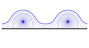
3.2. The von Kármán vortex streets travelling beneath a free surface in deep water

Following similar steps, analytical solutions for von Kármán vortex streets travelling beneath a free surface in deep water can be found. In the case of a so-called symmetric, or unstaggered, vortex street comprising two point vortex rows stacked vertically without any offset in the $x$ direction, this is the periodic wave analogue of the solitary wave just considered in § 3.1 since it can be viewed as a periodic array of point vortex pairs. Again the conformal mapping is denoted by $z=Z(\zeta )$ but now

(3.33)\begin{equation} Z'(\zeta) = \frac{{\rm i} R}{\zeta} \left ( \frac{(\zeta-c) (\zeta-d)}{(\zeta-a) (\zeta-b) } \right )^2,\quad a,b, R \in \mathbb{R},\enspace a, |b| > 1. \end{equation}

In the first instance both $a$ and $b$ will be chosen to be positive. Suppose it is required that, on integration,

(3.34)\begin{equation} Z(\zeta) = \frac{{\rm i}}{2{\rm \pi}} \left ( \log \zeta + \frac{A}{\zeta-a} + \frac{B}{\zeta-b} \right )+ Z_0, \end{equation}

for some real $A$ and $B$; the constant $Z_0$ can be chosen to ensure that $Z(1/a)=0$, say, which places the upper point vortex in a principal period window at the origin. In (3.34) the period of the waves has been chosen to be 1. For consistency between (3.33) and (3.34) it is necessary that

(3.35)\begin{equation} \frac{1}{2{\rm \pi}} = R \left (\frac{c d}{a b} \right )^2, \end{equation}

which gives $R$ in terms of the other parameters. The integrability requirements mean that the zeros $c$ and $d$ must be certain explicit functions of $a$ and $b$; these will be determined shortly. Supposing that suitable zeros $c$ and $d$ can be found, on differentiation of (3.34),

(3.36)\begin{equation} Z'(\zeta) = \frac{{\rm i}}{2{\rm \pi}} \left ( \frac{1}{\zeta} - \frac{A}{(\zeta-a)^2} - \frac{B}{(\zeta-b)^2} \right ), \end{equation}

so that, on equating the strengths of second-order poles between (3.33) and (3.36), it is necessary that

(3.37a,b)\begin{equation} \frac{{\rm i} R}{a} \left ( \frac{(a-c) (a-d)}{(a-b) } \right )^2 ={-} \frac{{\rm i} A}{2 {\rm \pi}},\quad \frac{{\rm i} R}{b} \left ( \frac{(b-c) (b-d)}{(b-a) } \right )^2={-} \frac{{\rm i} B}{2 {\rm \pi}} \end{equation}

which determine $A$ and $B$ in terms of $R,a,b,c$ and $d$. In order that $Z'(\zeta )$ integrates to give a simple pole of $Z(\zeta )$ at $\zeta =a$ then

(3.38)\begin{equation} \frac{2}{a - c} + \frac{2}{a-d} - \frac{1}{a} - \frac{2}{a-b} = 0. \end{equation}

Similarly, in order that $Z'(\zeta )$ integrates to give a simple pole of $Z(\zeta )$ at $\zeta =b$,

(3.39)\begin{equation} \frac{2}{b - c} + \frac{2}{b-d} - \frac{1}{b} - \frac{2}{b-a} = 0. \end{equation}

After some algebra, it can be shown that explicit solutions of the nonlinear equations (3.38) and (3.39) are

(3.40)\begin{equation} c = \frac{6ab- (a^2 +b^2) + {\rm i} (a-b)\sqrt{12ab-(a-b)^2}}{2(a+b)} = \bar{d}. \end{equation}

The velocity field is then given, as an explicit function of $\zeta$, by

(3.41)\begin{align} u - {\rm i} v = q \sqrt{S'(z)} = q \left ( - \frac{\zeta^{{-}1} \bar{Z}'(1/\zeta)}{\zeta Z'(\zeta) } \right )^{1/2}= q \frac{(1-\bar{c} \zeta) (1-\bar{d} \zeta)}{(1-a\zeta) (1-b \zeta) }\times \frac{(\zeta-a) (\zeta-b)}{(\zeta-c) (\zeta-d)}, \end{align}

where (3.33) has been used. It is clear that $u-{\rm i}v$ has two simple poles inside the fluid region at the images of $\zeta =1/a$ and $1/b$; these correspond to the two point vortices in each period window at $z_a=Z(1/a)$ and $z_b=Z(1/b)$.

The circulations $\varGamma _a$ and $\varGamma _b$ can now be found, after some algebra, to be

(3.42)\begin{gather} \varGamma_a = 2 {\rm \pi}qR \frac{(1-ca) (1-da)}{(1-a^2) (1-ba) } \frac{(1-\bar{c}/a) (1-\bar{d}/a)}{(1-b/a) }, \end{gather}

(3.43)\begin{gather}\varGamma_b = {2 {\rm \pi}q R} \frac{(1-cb) (1-db)}{(1-ab) (1-b^2) } \frac{(1-\bar{c}/b) (1-\bar{d}/b)}{(1-a/b) }. \end{gather}

It is natural to set the time scale of the flow by picking $q$ so that $\varGamma _a=1$. The value of $\varGamma _b$ required for the relative equilibrium then follows from (3.43). It follows from (3.41) that, as $\zeta \to 0$, or $y \to -\infty$,

(3.44)\begin{equation} u - {\rm i}v \to \frac{q a b}{cd} ={-}U, \end{equation}

where $U$ is the wave speed; recall that we have moved to a frame of reference cotravelling with the wave at speed $U$. For a given value of $a$ the value of $b$ can be found by specifying the vertical separation, $d$ say, of the two point vortices. This can be done by a simple Newton method, for example. The non-dimensional parameter $d/L$ relating the vertical separation of the two vortex rows making up a von Kármán vortex street to their period $L$ is referred to as the street aspect ratio (Saffman 1992). Since $L=1$ then $d$ corresponds to the aspect ratio of the street.

Figure 4 shows typical streamline distributions for different values of $a$ when $d=0.3$.

Figure 4. Symmetric (or unstaggered) von Kármán vortex streets of aspect ratio $d=0.3$ cotravelling with a free surface wave in deep water. Just two periods of the waves for $a=2, 1.25$ and $1.1$ are shown.

Figure 5 shows $\varGamma _b$ and $-U$ against $a$ for street aspect ratio $d=0.4$; this is typical of the graphs for other aspect ratios. As $a \to 1^+$ the speed $U$ tends to $1/(2{\rm \pi} d) \approx 0.397$ which is the magnitude of the azimuthal speed around a $d$-radius circle centred at an isolated unit-circulation point vortex. Thus, as for the single pair generating a solitary wave in § 3.1, the flow in this limit comprises a periodic array of point vortices each with a near circular orbit of irrotational fluid rolling on a flat interface. On the other hand, as $a \to \infty$, $U$ tends to the speed of the symmetric von Kármán vortex street as given by

(3.45)\begin{equation} \frac{\varGamma}{2L} \coth \left ( \frac{{\rm \pi} d}{L} \right ). \end{equation}

This is the speed of a symmetric von Kármán vortex street, with one point vortex row of period $L$ made up of vortices of circulation $\varGamma$ situated a vertical distance $d$ above a similar row with vortices of circulation $-\varGamma$ (Saffman 1992). In this case with $\varGamma =L=1$, $U \to (1/2)\coth ({\rm \pi} d)$ and this value is expected because as $a \to \infty$ the wave interface moves up in the positive $y$-direction meaning that its effect on the vortex street becomes gradually negligible and the street travels at its free-space value as first computed by von Kármán (Saffman 1992).

Figure 5. Graphs of $\varGamma _b$ and $-U$ as functions of $a$ for a symmetric von Kármán vortex street beneath a free surface. As $a \to 1^+$ the wave speed $U$ tends to $1/(2{\rm \pi} d) \approx 0.397$; as $a \to \infty$, $U$ tends to $0.588$ which corresponds to the speed of the symmetric von Kármán vortex street given by (3.45) for $\varGamma =L=1,\ d=0.4$.

Finally, if $a> 1$ but $b < -1$ then the point vortices in the two rows correspond to an asymmetric (or staggered) von Kármán vortex street beneath a free surface: this is where one vortex row is now offset (staggered) relative to the other by half a period in the $x$ direction. All the same formulas given above pertain and graphs akin to those shown in figure 5 can easily be drawn. Figure 6 shows a typical streamline plot for a periodic wave on an interface cotravelling with such a submerged staggered von Kármán vortex street. In this case, for the chosen $a=4$ the appropriate negative value of $b$ has been found giving $d=0.4$ as the aspect ratio of the submerged staggered street.

Figure 6. An asymmetric, or staggered, von Kármán vortex street of aspect ratio $d=0.4$ cotravelling with a free surface wave in deep water.

4. More exotic waves

It is natural to ask about the possibility of adding more point vortices per period. As will now be shown, the case of 3 point vortices per period has some intriguing connections with certain ‘exotic waves’ that have been computed numerically for constant vorticity (Vanden-Broeck 1996; Hur & Dyachenko 2019a,b; Hur & Vanden-Broeck 2020). Let the derivative of the conformal mapping now have the form

(4.1)\begin{equation} Z'(\zeta) = \underbrace{\frac{{\rm i} R}{\zeta} \left(\frac{\zeta-c}{\zeta-a}\right)^2}_{\text{Crowdy & Roenby (2014)}} \underbrace{\left[\frac{(\zeta-\gamma) (\zeta-\bar{\gamma})}{(\zeta-b) (\zeta-d)}\right]^2}_{\text{near-circular apex wave}}, \end{equation}

where $b, c, d\in \mathbb {R}$ and $\gamma$ is complex. Besides being of the functional form that will potentially allow for case 2 equilibria, the rationale for the functional form (4.1) is as follows. The first term in the product representation in (4.1) is precisely that found by Crowdy & Roenby (2014) to correspond to a single point vortex row beneath a free surface. This expression has been multiplied by a term with two simple poles at $b$ and $d$, taken to be on the real axis close to $\zeta =1$, which is the preimage of the apex of the Crowdy–Roenby wave, and also has two simple zeros at complex conjugate positions $\gamma \in \mathbb {C}$ and $\bar {\gamma }$. The reason for adding this term is to seek a case 2 wave resembling the constant-vorticity wave comprising a Crowdy–Roenby wave with a superposed near-circular wave akin to that found numerically in the constant-vorticity case by Vanden-Broeck (1996) and Hur & Vanden-Broeck (2020). If $b,d, \gamma$ and $\bar {\gamma }$ are all near unity then for values of $\zeta$ away from $\zeta =1$, the free surface profiles are expected to resemble a Crowdy–Roenby wave. Only the image of $\zeta$-points close to $\zeta =1$ will differ substantially from this. Moreover, the nearest simple pole is expected to induce a near-circular wave as the form of this localized disturbance near the apex of the wave, with the two zeros at $\gamma$ and $\bar {\gamma }$ furnishing the preimages of the two near-cuspidal sides of the tightening neck joining this near-circular wave to the Crowdy–Roenby wave beneath it.

The question remains as to whether parameters generally fitting these stipulations also allow for the steadiness requirements that $S(z)$ has simple pole singularities, and therefore no logarithmic singularities, at the point vortex locations $z_a=Z(1/a),\ z_b=Z(1/b)$ and $z_d=Z(1/d)$. These integrability conditions are equivalent to $Z(\zeta )$ having simple poles at $\zeta =a,b,d$ and that requires

(4.2)\begin{gather} \frac{2}{a-c} + \frac{2}{a-\gamma} + \frac{2}{a-\bar{\gamma}} = \frac{1}{a} + \frac{2}{a-b} + \frac{2}{a-d}, \end{gather}

(4.3)\begin{gather}\frac{2}{b-c} + \frac{2}{b-\gamma} + \frac{2}{b-\bar{\gamma}} = \frac{1}{b} + \frac{2}{b-a} + \frac{2}{b-d}, \end{gather}

(4.4)\begin{gather}\frac{2}{d-c} + \frac{2}{d-\gamma} + \frac{2}{d-\bar{\gamma}} = \frac{1}{d} + \frac{2}{d-a} + \frac{2}{d-b}. \end{gather}

If parameters satisfying these conditions can be found, the mapping integrates to the following log-rational function:

(4.5)\begin{equation} z = Z(\zeta) = \frac{{\rm i}}{2{\rm \pi}} \log \zeta + \frac{{\rm i} A}{\zeta-a}+ \frac{{\rm i} B}{\zeta-b} + \frac{{\rm i} D}{\zeta-d}, \end{equation}

where we pick $R$ such that

(4.6)\begin{equation} R \left(\frac{c \gamma \bar{\gamma}}{a b d} \right )^2 = \frac{1}{2{\rm \pi}}, \end{equation}

and then

(4.7)\begin{align} \left.\begin{gathered} A ={-}\frac{R}{a} \left (\frac{ (a-c)(a-\gamma)(a-\bar{\gamma})}{(a-b)(a-d)} \right )^2,\quad B ={-}\frac{R}{b} \left (\frac{ (b-c)(b-\gamma)(b-\bar{\gamma})}{(b-a)(b-d)} \right )^2, \\ D ={-}\frac{R}{d} \left (\frac{ (d-c)(d-\gamma)(d-\bar{\gamma})}{(d-a)(d-b)} \right )^2, \end{gathered}\right\} \end{align}

where, to establish (4.7), the second-order pole strengths of (4.1) and the derivative of (4.5) have been equated. It turns out that such parameters can indeed be found: the three real parameters $a, b$ and $d$ can be selected and (4.2)–(4.4) solved for the corresponding $c$ and $\gamma$ (three real unknowns because $c$ is real valued and $\gamma$ is complex valued). This was done numerically. Once suitable parameters are found the solutions for the wave shape, point vortex circulations and the velocity field are known in analytical form. Incidentally, even when solutions of (4.2)–(4.4) can be found, not all choices of $a, b$ and $d$ yield solutions for $c$ and $\gamma$ that furnish univalent mappings corresponding to physically admissible waves.

Figure 7 shows two such steadily propagating waves corresponding to ${a=2.3}, {b=1.002}, {d=1.0429}$ and $a=2.3, b=1.0001, d=1.0096$. In each case, $b$ and $d$ have been chosen close to unity. Typically, it is found that if $b=1+\epsilon$ where $\epsilon \ll 1$ then choosing $d= 1+{O}(\epsilon ^{1/2})$ will generally produce the class of shapes qualitatively resembling those found for weak gravity by Vanden-Broeck (1996) (see his figure 5c) and Hur & Vanden-Broeck (2020) (see their figure 8); moreover, the zeros $\gamma$ and $\bar {\gamma }$ are also found to be close to $\zeta =1$. The circulations at $z_a = Z(1/a), z_d = Z(1/d)$ and $z_b=Z(1/b)$, corresponding to the lower, middle and upper point vortex respectively, are given by

(4.8)\begin{equation} \left.\begin{gathered} \varGamma_a = 2 {\rm \pi}q R{(1-c/a) }\frac{(a-\gamma) (a- \bar{\gamma})}{(a- b)(a-d)} \frac{(1-ca)}{(1-a^2)}\frac{(1-a \gamma) (1-a \bar{\gamma})}{(1-ab)(1-ad)}, \\ \varGamma_b =2 {\rm \pi}q R {(1-c/b)}\frac{(b-\gamma) (b- \bar{\gamma})}{(b-a)(b-d)} \frac{(1-bc)}{(1-ab)}\frac{(1-b\gamma) (1-b\bar{\gamma})}{(1-b^2)(1-bd)},\\ \varGamma_d =2 {\rm \pi}qR{(1-c/d) }\frac{(d-\gamma) (d- \bar{\gamma})}{(d-a)(d- b)} \frac{(1-cd)}{(1-ad)} \frac{(1-d \gamma) (1-d\bar{\gamma})}{(1-bd)(1-d^2)}. \end{gathered}\right\} \end{equation}

If $q$ is chosen so that $\varGamma _a=1$ then the corresponding values of $\varGamma _b$ and $\varGamma _d$ can be determined. For the two example waves shown in figure 7 the circulations are ${\varGamma _a=1}, {\varGamma _d = -0.1253}, {\varGamma _b =0.9679}$ and $\varGamma _a=1, \varGamma _d = -0.0308, \varGamma _b =1.0026$, respectively. Notice that the value of $\varGamma _d$, the circulation of the point vortex sitting in the necking region, gets smaller as $b$ gets closer to unity. This is the same phenomenon as observed for the solitary wave found in § 3.1.

Figure 7. Steadily translating waves with 3 point vortices per period (two periods are shown). (a) The image of the mapping (4.1) for $a=2.3,\ b=1.002,\ d=1.0429$ with $\varGamma _a=1,\ \varGamma _d = -0.1253, \varGamma _b =0.9679$; (b) $a=2.3,\ b=1.0001,\ d=1.0096$ with $\varGamma _a=1,\ \varGamma _d = -0.0308,\ \varGamma _b =1.0026$. The point vortex locations are indicated by dots. In the period window on the left the Crowdy & Roenby (2014) profile for $a=2.3$ is superposed for comparison. The waves qualitatively resemble those found for weak gravity and constant vorticity by Hur & Vanden-Broeck (2020).

Figure 7 provides evidence that case 2 equilibria exist comprising irrotational waves with 3 cotravelling point vortices per period that have profiles highly reminiscent of similar near-zero-gravity travelling waves with constant vorticity as computed numerically by Vanden-Broeck (1996) and Hur & Vanden-Broeck (2020). Moreover, close to the limiting waves comprising a near-circular wave atop a Crowdy–Roenby wave, the circulation of the point vortex in the necking region becomes vanishingly small suggesting that the case 2 analogues of the constant-vorticity waves at zero gravity in Vanden-Broeck (1996) and Hur & Vanden-Broeck (2020) have two point vortices per period, one associated with the Crowdy–Roenby wave, a second with the near-circular wave sitting atop it. We conjecture that generalized case 2 exotic waves, with successively more circular waves piling on top of each other, as occurs for constant-vorticity waves with weak gravity as shown by Hur & Dyachenko (2019b), can be constructed by successively including additional poles in the rational function (4.1) and then solving for the associated zeros that ensure integrability without logarithms at the poles.

5. Point vortex row in a fluid sheet

Another question is whether case 2 steadily travelling waves can be found on fluid of finite depth. The answer is in the affirmative. Solutions have been found both for a single point vortex cotravelling with a solitary wave in fluid of finite depth, and for a point vortex row cotravelling with a periodic wave on finite-depth fluid. Moreover, both solutions can be found in analytical form, although the latter solution requires some more sophisticated mathematical technology that will be explained in this section. It turns out that another solution of fluid dynamical interest can be constructed using those same new techniques: it does not involve a travelling wave but is an equilibrium wherein a vortex row sits between two symmetric free surfaces, or in a fluid sheet, providing a model of a rolled-up shear layer. This solution will be presented first, both for completeness, and because its functional form is more basic than the solution for periodic travelling waves to be presented in § 7 and therefore affords a simpler context in which to introduce the required theoretical elements.

The new tool is the prime function of a concentric annulus $\rho < |\zeta | < 1$ (Crowdy et al. 2016). Only the essential properties of this function needed to construct the solutions of interest here will be given. In fact, the requisite tools are exactly those used by Crowdy & Green (2011) to construct analytical solutions for von Kármán streets of hollow vortices; see also Crowdy & Krishnamurthy (2017). Readers interested in more details of the general theory of the prime function associated with a multiply connected domain can refer to a recent monograph on this topic (Crowdy 2020).

Consider a $2{\rm \pi}$-periodic point vortex row situated along the centreline of a fluid sheet where the upper surface is the reflection in the real axis of the lower surface of the sheet. Since the fluid velocity on the upper and lower surfaces is expected to be of the same magnitude but in opposite directions it is expected that

(5.1)\begin{equation} u + {\rm i}v = \left \lbrace \begin{array}{ll} q \displaystyle\dfrac{{\rm d} {z}}{{\rm d} s} & {\rm on\ the\ upper\ surface}, \\ q \displaystyle\dfrac{{\rm d} {z}}{{\rm d} s} & {\rm on\ the\ lower\ surface}, \\ \end{array}\right . \end{equation}

where, as before, $dz/ds$ denotes the complex unit tangent with arclength increasing with fluid to the right as the boundary of the period window is traversed. It is known, from an extension of the Riemann mapping theorem (Crowdy 2020), that the concentric annulus $\rho < |\zeta | < 1$ provides a suitable preimage for a conformal mapping of the general form

(5.2)\begin{equation} z = Z(\zeta) = {\rm i} \log \zeta + {\rm function\ analytic\ in\ the\ annulus} \end{equation}

to a single period of the fluid region. The branch cut of the logarithm can be taken along the negative real $\zeta$ axis. The upper and lower sides of this branch cut are transplanted to the two sides of a principal period window of the configuration, as indicated in figure 8.

Figure 8. Conformal mapping from the concentric annulus $\rho < |\zeta | < 1$ in a parametric $\zeta$ plane to a single period of a wave on a fluid sheet of finite depth in the physical $z$ plane. The two sides of a logarithmic branch cut along the negative real $\zeta$ axis, say, are transplanted to the two sides of the period window. For all flows considered in this paper, a reflectional symmetry of the two interfaces about the real $z$-axis means that the preimage of the latter is the circle $|\zeta | =\sqrt {\rho }$ in the $\zeta$ annulus (dotted lines).

On the boundary circle $|\zeta |=1$, the familiar formula

(5.3)\begin{equation} \frac{{\rm d}\bar{z}}{{\rm d} s} = \left ( -\frac{ \zeta^{{-}1} \bar{Z}'(\zeta^{{-}1})}{\zeta Z'(\zeta)} \right )^{1/2} \end{equation}

pertains. However, this has a modified form on $|\zeta |=\rho$ given by

(5.4)\begin{equation} \frac{{\rm d}\bar{z}}{{\rm d} s} ={-} \left ( -\frac{ \rho^2 \zeta^{{-}1} \bar{Z}'(\rho^2 \zeta^{{-}1})}{\zeta Z'(\zeta)} \right )^{1/2}. \end{equation}

If we define the function

(5.5)\begin{equation} F(\zeta) = (\zeta Z'(\zeta))^{1/2} ,\end{equation}

then from the complex conjugate of (5.1), and considering the case 2 scenario where the meromorphic continuation of $\textrm {d}\bar {z}/\textrm {d} s$ into the fluid domain gives $u-\textrm {i} v$, it can be seen that a consistent irrotational flow in the fluid domain between the two free surfaces will be defined by meromorphic continuation if

(5.6)\begin{equation} F(\rho^2 \zeta) ={-} F(\zeta). \end{equation}

This requirement ensures that the meromorphic continuation of $\textrm {d} \bar {z}/\textrm {d} s$ from $|\zeta |=1$ into the fluid coincides with the meromorphic continuation of $\textrm {d} \bar {z}/\textrm {d} s$ from $|\zeta |=\rho$ into the fluid, and that both will produce consistent expressions for $u-\textrm {i}v$. For a single point vortex per period, these continuations off the boundary circles will have a single simple pole inside the annulus and, being the same, will give a well-defined irrotational flow involving a point vortex row.

The prime function of the annulus $\rho < |\zeta | < 1$ can be defined, for $0 \le \rho < 1$, as

(5.7a,b)\begin{equation} P(\zeta, \rho) = (1-\zeta) \hat P(\zeta,\rho),\quad \hat P(\zeta,\rho) = \prod_{n=1}^\infty (1-\rho^{2n} \zeta) (1-\rho^{2n} /\zeta). \end{equation}

This infinite product representation of $P(\zeta,\rho )$ is convergent for $0 \le \rho < 1$, and adequate for the purposes of this paper, but there are alternative ways to compute it (Crowdy 2020). This function has a simple zero when $\zeta =1$ (and, in fact, other simple zeros at $\zeta =\rho ^{2n}$ for $n \in \mathbb {Z}$). It is a simple exercise to verify, directly from its infinite product definition, that $P(\zeta,\rho )$ satisfies the functional relations

(5.8a,b)\begin{equation} P(\zeta^{{-}1},\rho) ={-}\zeta^{{-}1} P(\zeta,\rho),\quad P(\rho^2 \zeta,\rho) ={-}\zeta^{{-}1} P(\zeta,\rho). \end{equation}

It is also useful to introduce a logarithmic derivative of this function defined by

(5.9a,b)\begin{equation} K(\zeta,\rho) = \zeta \frac{P'(\zeta,\rho)}{P(\zeta,\rho)} ={-} \frac{\zeta}{\zeta-1} + \hat K(\zeta,\rho),\quad \hat K(\zeta,\rho) = \zeta \frac{\hat P'(\zeta,\rho)}{\hat P(\zeta,\rho)}, \end{equation}

where the prime notation denotes differentiation with respect to the first argument of the function. An important feature is that $K(\zeta,\rho )$ has a simple pole at $\zeta =1$ (and, in fact, at $\zeta =\rho ^{2n}$ for $n \in \mathbb {Z}$). Two functional relations deriving from (5.8a,b) are

(5.10a,b)\begin{equation} K(\zeta^{{-}1},\rho) = 1-K(\zeta,\rho),\quad K(\rho^2 \zeta,\rho) = K(\zeta,\rho) -1. \end{equation}

Finally, another derivative will be needed here. Let

(5.11)\begin{equation} L(\zeta,\rho) = \zeta K'(\zeta,\rho) \end{equation}

which can be verified to satisfy the two functional relations

(5.12a,b)\begin{equation} L(\zeta^{{-}1},\rho) = L(\zeta,\rho),\quad L(\rho^2 \zeta,\rho) = L(\zeta,\rho). \end{equation}

These are the function theoretic tools required to build the solutions.

Let

(5.13)\begin{equation} \zeta Z'(\zeta) = {\rm i} C \left(\frac{P(-\zeta \sqrt{\rho},\rho)}{P(\zeta \sqrt{\rho},\rho)}\right)^2 \end{equation}

for some real constant $C$; this has a double zero at $\zeta =-1/\sqrt {\rho }$ and a double pole at $\zeta =1/\sqrt {\rho }$, both of which are outside the annulus $\rho < |\zeta | < 1$. Clearly,

(5.14)\begin{equation} F(\zeta) = ({\rm i} C)^{1/2} \frac{P(-\zeta \sqrt{\rho},\rho)}{P(\zeta \sqrt{\rho},\rho)} \end{equation}

and it can be checked, using the properties (5.8a,b) of $P(\zeta,\rho )$, that this satisfies (5.6). It is necessary to check that this function integrates to give a simple pole at $1/\sqrt {\rho }$. Let

(5.15)\begin{equation} Z'(\zeta) = \frac{{\rm i} C}{\zeta} \left(\frac{P(-\zeta \sqrt{\rho},\rho)}{P(\zeta \sqrt{\rho},\rho)} \right )^2 = \frac{X(\zeta)}{(\zeta-1/\sqrt{\rho})^2}, \end{equation}

where

(5.16)\begin{equation} X(\zeta) \equiv \frac{{\rm i} CP^2(-\zeta \sqrt{\rho}, \rho)}{\rho \zeta \hat P^2(\zeta \sqrt{\rho},\rho)}. \end{equation}

The integrability condition at $\zeta =1/\sqrt {\rho }$ requires that

(5.17)\begin{equation} X'(1/\sqrt{\rho}) = 0. \end{equation}

But

(5.18)\begin{equation} \frac{\zeta X'(\zeta)}{X(\zeta)} ={-}1 + 2 K(-\zeta \sqrt{\rho},\rho) - 2 \hat K(\zeta \sqrt{\rho},\rho), \end{equation}

and since, from (5.7a,b) and (5.9a,b),

(5.19)\begin{equation} K(\zeta,\rho)={-} \frac{\zeta}{1-\zeta} + \hat K(\zeta,\rho) ={-} \frac{\zeta}{1-\zeta} - \sum_{n=1}^\infty \frac{\rho^{2n} \zeta}{1-\rho^{2n}\zeta} +\sum_{n=1}^\infty \frac{\rho^{2n}/\zeta}{1-\rho^{2n}/\zeta} \end{equation}

then it is easy to check that

(5.20a,b)\begin{equation} K({-}1,\rho) = \tfrac{1}{2},\quad \hat K(1,\rho) = 0, \end{equation}

which confirms that (5.17) indeed holds. It can then be inferred (Crowdy 2020) that

(5.21)\begin{equation} Z(\zeta) = {\rm i} A \log \left (\frac{\zeta}{\sqrt{\rho}} \right ) + {\rm i}B (K(\zeta \sqrt{\rho}, \rho) - K(\rho, \rho)), \end{equation}

for some $B$ and where a constant of integration has been chosen to ensure that $\zeta =\sqrt {\rho }$ corresponds to the origin in the $z$ plane. Recall that $K(\zeta \sqrt {\rho }, \rho )$ has a simple pole at $\zeta =1/\sqrt {\rho }$. For a given $A$, the constant $B$ must be picked so that $\zeta Z'(\zeta )$ as computed by taking a derivative of (5.21), i.e.

(5.22)\begin{equation} \zeta Z'(\zeta) = {\rm i} A + {\rm i}B L(\zeta \sqrt{\rho}, \rho), \end{equation}

vanishes when $\zeta =-1/\sqrt {\rho }$, as required for consistency with (5.13). Thus,

(5.23)\begin{equation} A + BL({-}1, \rho) = 0. \end{equation}

The constant $C$ is directly relatable to $B$ by equating second-order pole strengths at $1/\sqrt {\rho }$. Specifically, choosing $A=1$ so that the waves are $2 {\rm \pi}$-periodic then we have two different but equivalent formulas for the derivative of the conformal mapping, namely

(5.24)\begin{equation} \zeta Z'(\zeta) = {\rm i} \left (1 + B L(\zeta \sqrt{\rho}, \rho) \right ) = {\rm i} C \left ( \frac{P(-\zeta \sqrt{\rho},\rho)}{P(\zeta \sqrt{\rho},\rho)} \right )^2, \end{equation}

where, from (5.23) and by equating the second-order pole strengths in (5.24),

(5.25a,b)\begin{equation} B ={-} \frac{1}{L({-}1,\rho)},\quad C ={-} B \left ( \frac{\hat P(1,\rho)}{P({-}1,\rho)} \right )^2 = \left(\frac{\hat P(1,\rho)}{P({-}1,\rho)} \right )^2 \frac{1}{L({-}1,\rho)}. \end{equation}

The case 2 velocity field is then

(5.26)\begin{equation} u-{\rm i}v = q \left (-\frac{\zeta^{{-}1} \bar{Z}'(\zeta^{{-}1})}{\zeta Z'(\zeta)} \right )^{1/2} = q \left(\frac{P(- \sqrt{\rho}/\zeta,\rho)}{P( \sqrt{\rho}/\zeta,\rho)} \right ) \left(\frac{P(\zeta \sqrt{\rho},\rho)}{P(-\zeta \sqrt{\rho},\rho)} \right ) \end{equation}

which, because of the simple pole singularity in the annulus $\rho < |\zeta | < 1$ at $\zeta =\sqrt {\rho }$ corresponding to $z=0$, gives the flow associated with an equilibrium point vortex row equilibrium between two free surfaces because $\sqrt {S'(z)}$ and $S(z)$ have all the required properties for equilibrium. By a local expansion, the circulation $\varGamma$ of each point vortex is found to be given by

(5.27)\begin{equation} \varGamma ={-}2 {\rm \pi}q C \left(\frac{P(-\rho,\rho)P({-}1,\rho)}{P(\rho,\rho) \hat P(1,\rho)}\right). \end{equation}

The time scale of the flow can be set, for example, by picking $\varGamma =1$ which determines $q$ according to (5.27) leaving a one-parameter family of solutions parametrized by $\rho$. The value of $\rho$ determines the depth of the fluid per period and the infinite-depth limit corresponds to taking $\rho \to 0$, in which case, the annulus $\rho < |\zeta | < 1$ reduces to the unit disc. In principle, the mathematical parameter $\rho$ could be removed by finding the value of it corresponding to some specified value of the average fluid layer depth, but use of $\rho$ is found to be more convenient. Figure 9 illustrates some typical solutions.

Figure 9. Streamlines and equilibrium free surfaces associated with a periodic vortex row in a finite-depth fluid sheet for $\rho =0.005, 0.05$ and $0.2$. These solutions are not travelling waves but steady equilibria. The characteristic ‘cat's-eye’ streamlines typical of a rolled-up shear layer are evident.

Properly arguing for some of the mathematical steps above requires use of the function theory expounded in Crowdy (2020) – ideas also used in Crowdy & Green (2011) and Crowdy & Krishnamurthy (2017) – but the reader can readily check numerically the validity of the formulas reported above.

A straightforward analysis can be used to confirm that, as $\rho \to 0$, then $\zeta /\sqrt {\rho } \to \textrm {e}^{-\textrm {i}z}$ and, from (5.26),

(5.28)\begin{equation} u - {\rm i} v \to {\rm i} q \cot(z/2), \end{equation}

which is the familiar complex velocity field associated with a single $2{\rm \pi}$-periodic point vortex row of circulation $-4 {\rm \pi}q$ in free space with no free surfaces present. Therefore, this new class of solutions is a generalization of this simple solution for a point vortex row in an unbounded fluid to the situation where the point vortex row is now situated in a finite-depth fluid sheet with symmetric top and bottom free surfaces.

6. Solitary wave incited by a point vortex in water of finite depth

Before proceeding to the problem of a periodic point vortex row in a finite-depth layer, it is natural to ask first about a single point vortex cotravelling with a solitary wave.

Consider the problem of a single point vortex pair, of equal and opposite circulations at $(0,\pm 1)$, in a fluid layer of finite depth. Solutions for which the two free surfaces are identical in shape, and reflections of each other about the $x$ axis will be sought. Then the $x$ axis is expected to be a streamline of the flow and the problem is equivalent to the problem of a point vortex beneath a free surface in water of finite depth with a flat impenetrable bottom wall.

Since this is a solitary wave solution, and the free surfaces can be thought of as meeting at $x \to \pm \infty$, then the annulus is not needed: the unit disc $|\zeta | < 1$ is sufficient to parametrize the fluid domain provided that two logarithmic singularities of the mapping $z=Z(\zeta )$, at $\zeta = \pm 1$ say, are admitted on the unit circle. Let

(6.1)\begin{equation} Z'(\zeta) = \frac{R}{\zeta^2-1} \left ( \frac{\zeta^2-c^2}{\zeta^2+a^2} \right )^2,\ a, R \in \mathbb{R} \end{equation}

which has the requisite simple poles at $\zeta =\pm 1$ which will produce logarithmic singularities of the mapping $Z(\zeta )$ at $\zeta = \pm 1$. This function has two second-order poles at $\zeta =\pm \textrm {i} a$ which are preimages of two point vortices in the fluid layer. For these to be in equilibrium the condition that the mapping has simple poles at ${\pm }\textrm {i} a$, and not logarithmic singularities, is

(6.2)\begin{equation} c= \frac{a^2(a^2+3)}{3 a^2+1}. \end{equation}

With this choice the mapping function is

(6.3)\begin{equation} Z(\zeta) = R \left [ \frac{1}{2} \left (\frac{1-c^2}{1+a^2} \right )^2 \log \left (\frac{1-\zeta}{1+\zeta} \right ) - \frac{2}{a^2+1} \left (\frac{a^2 +c^2}{2a} \right )^2 \frac{\zeta}{\zeta^2+a^2} \right ]. \end{equation}

The associated velocity field is

(6.4)\begin{equation} u - {\rm i} v = q\frac{(1-c^2 \zeta^2)(\zeta^2+a^2)}{(1+a^2 \zeta^2)(\zeta^2-c^2)}. \end{equation}

The constant $R$ can be chosen so that $Z(\textrm {i}/a)=\textrm {i}$ thereby setting the length scale of the problem and $q$ can be chosen so that the circulation of the point vortex at this location is unity thereby setting the time scale of the flow. The result is a one-parameter family of equilibrium solutions parametrized by $a$.

Figure 10 shows three typical wave profiles for $a=4, 2$ and $1.5$ and reveals how the profile becomes more distorted as $a$ gets closer to unity. These solitary wave solutions would appear to be analogues of solitary waves, with strong uniform vorticity compared with a weaker gravity effect, found recently by Kozlov, Kuznetsov & Lokharu (2020).

Figure 10. Typical solitary waves incited by a travelling point vortex in water of finite depth. The cases $a=4, 2$ and $1.5$ of a one-parameter family of waves are shown.

This problem has similarities with that of a point vortex in an open jet flow near a solid boundary for which exact solutions have been derived by Gurevich (1963) and Shaw (1972) who found analytical solutions for an irrotational streaming flow, in water of finite depth, over a point vortex. Doak & Vanden-Broeck (2017) have studied this class of problems numerically, including the effect of gravity. Unlike the new solution just derived, however, the point vortex in all the solutions just mentioned is not free but has an external force on it making it a somewhat different problem.

7. Periodic waves incited by a point vortex row in finite-depth water

As a final example, the problem of a periodic point vortex row travelling steadily in a fluid layer of finite depth with a flat impenetrable lower wall will be addressed. In this case, the prime function machinery associated with the annulus $\rho <|\zeta | <1$ given in § 5 is once again needed to parametrize the solutions. And as in § 6, solutions for which the two free surfaces are identical in shape, and reflections of each other about the $x$ axis, will be sought. Once solved, only the flow in $y > 0$ will be examined corresponding to a single point vortex row in a finite-depth fluid layer, the $x$-axis line of symmetry being a streamline of the flow and interpreted as the flat impenetrable lower wall of the fluid layer.

There is now a sign difference compared with condition (5.1) relevant to a single vortex row in a fluid sheet because, for steadily travelling waves involving two vortex rows, it is expected that

(7.1)\begin{equation} u + {\rm i}v = \left \lbrace \begin{array}{ll} +q \displaystyle\dfrac{{\rm d} {z}}{{\rm d} s} & {\rm on\ the\ upper\ surface}, \\ -q \displaystyle\dfrac{{\rm d} {z}}{{\rm d} s} & {\rm on\ the\ lower\ surface}. \end{array}\right. \end{equation}

This is because the velocity on the top and bottom interfaces generated by a pair of vortex rows each made up of vortices having equal strength, but opposite sign, circulations to be of the same magnitude and in the same direction. Therefore, in contrast to (5.6), it must now be arranged that

(7.2)\begin{equation} F(\rho^2 \zeta) = F(\zeta), \end{equation}

where $F(\zeta )$ is still defined as in (5.5).

Consider the conformal mapping $z=Z(\zeta )$ from the annulus $\rho < |\zeta |< 1$ with

(7.3)\begin{equation} \zeta Z'(\zeta) = {\rm i} D \left ( \frac{P(\zeta/\gamma,\rho) P(\zeta/\bar{\gamma},\rho)}{P(\zeta/a,\rho)P(\zeta a \rho, \rho)} \right )^2,\ D \in \mathbb{R} \end{equation}

where $1 < a < 1/\rho$ and take $\gamma =\textrm {e}^{\textrm {i} \theta }/\sqrt {\rho }$ where the real argument $\theta$ is to be determined. The image of the circle $|\zeta | =\sqrt {\rho }$ will correspond to the real axis in the $z$ plane, or the impenetrable lower wall about which the two wave profiles are reflectionally symmetric. Later, we will only be interested in the image of the sub-annulus $\sqrt {\rho } < |\zeta | < 1$ corresponding to a single period of the flow of a point vortex row in a fluid layer of finite depth. The derivative of the mapping (7.3) is analytic in $\rho < |\zeta |< 1$, as required, but it has two (second-order) poles outside this annulus at $\zeta =a$ and $1/(a\rho )$. Both of these poles are in the annulus $1 < |\zeta | < 1/\rho$ although the mapping actually has infinitely more image poles in many other annuli in the complex $\zeta$ plane. It is easy to verify, using the functional relations (5.8a,b), that $F(\zeta )$ as defined in (5.5), and determined now by (7.3), satisfies relation (7.2). It is for this reason that it is enough to restrict attention to its pole structure in the fundamental annulus $\rho < |\zeta | < 1/\rho$ since the pole structure in all other equivalent annuli will be inherited from this relation.

The function (7.3) is also a square of a meromorphic function so that the case 2 velocity field is

(7.4)\begin{equation} u - {\rm i} v = q \frac{P(1/(\zeta \gamma),\rho) P(1/(\zeta \bar{\gamma}),\rho)}{P(1/(\zeta a),\rho)P( a \rho/\zeta, \rho)} \frac{P(\zeta/ a,\rho)P(\zeta a \rho, \rho)}{P(\zeta/\gamma,\rho) P(\zeta/\bar{\gamma},\rho) }, \end{equation}

which has no square-root branch points but two simple poles in the annulus $\rho <|\zeta | < 1$ at $\zeta =1/a$ and $a \rho$; these are the pre-images of the two point vortices per period which are located at locations $Z(1/a)$ and $Z(a \rho )$ in the physical $z$-plane. It should be noted that the pole at $a \rho$ is the reflection of the pole at $1/a$ in the circle $|\zeta |=\sqrt {\rho }$ (which, it should be recalled, is the pre-image of the impenetrable lower wall of the fluid layer).

The integrability condition on $Z'(\zeta )$ at $a$ – namely, that its primitive $Z(\zeta )$ has no logarithmic singularity there – requires that

(7.5)\begin{equation} 2 K(a/\gamma,\rho) + 2 K(a/\bar{\gamma},\rho) - 2 \hat K(1,\rho) - 2 K(a^2 \rho,\rho) - {1} = 0. \end{equation}

But $\hat K(1,\rho ) =0$ so this condition reduces to

(7.6)\begin{equation} 2 K(a/\gamma,\rho) + 2 K(a/\bar{\gamma},\rho)- 2 K(a^2 \rho,\rho) - {1} = 0.\end{equation}

For a given $a$ and $\rho$, this can be solved for $\theta$ where $\gamma =\textrm {e}^{\textrm {i} \theta }/\sqrt {\rho }$. This is easily done using Newton's method. By the symmetry of this configuration, when this condition holds it can be shown, on use of the properties (5.10a,b), that the primitive $Z(\zeta )$ also has a simple pole at $1/(\rho a)$ meaning that no other equation needs to be solved to enforce this other requirement. This apparently fortunate circumstance is a consequence of symmetries built into the ansatz (7.3). With parameters chosen thus, it follows that (Crowdy 2020)

(7.7)\begin{equation} Z(\zeta) = {\rm i} \left ( \log \zeta + A (K(\zeta/a,\rho) + K(\zeta a \rho, \rho)) \right ) + Z_0,\quad Z_0 \in \mathbb{C}, \end{equation}

for some real $A \in \mathbb {R}$ and where the spatial period has been set to $2 {\rm \pi}$. The integration constant $Z_0$ can be selected so that the image of $|\zeta |=\sqrt {\rho }$ lies on $y=0$ in the $z$-plane. Recall the property that $K(\zeta,\rho )$ has a simple pole at $\zeta =1$ meaning that (7.7) has simple poles at $\zeta =a$ and $1/(a\rho )$, as required. The value of $A$ is determined by ensuring that

(7.8)\begin{equation} \zeta Z'(\zeta) = {\rm i} \left (1+ A (L(\zeta/a,\rho) + L(\zeta a \rho, \rho)) \right ), \end{equation}

vanishes at $\gamma$, i.e.

(7.9)\begin{equation} A={-} \frac{1}{L(\gamma/a,\rho) + L(\gamma a \rho, \rho)}, \end{equation}

which is needed on inspection of (7.3) which, using the properties (5.8a,b), has zeros (in the fundamental annulus) at $\zeta = \gamma, \bar {\gamma }$. The expression (7.8) is obtained by taking a derivative of (7.7) with respect to $\zeta$ and then multiplying by $\zeta$. Using the properties (5.12a,b) of $L(\zeta,\rho )$ it can be verified that $A$ is real. Then, on taking a complex conjugate of (7.8), it can be checked that if (7.8) has a simple zero at $\gamma$ then it has another at $\bar {\gamma }$, thereby enforcing another requirement apparent from (7.3). The relation between $A$ and $D$ is determined by equating the strengths of second-order poles at $\zeta =a$ between (7.3) and (7.8)

(7.10)\begin{equation} D ={-} A \left ( \frac{\hat P(1,\rho)P( a^2 \rho, \rho)}{P( a/\gamma,\rho) P( a/\bar{\gamma},\rho) } \right )^2. \end{equation}

Once again, the reader is referred to the general theory presented by Crowdy (2020) (see also Crowdy & Green 2011; Crowdy & Krishnamurthy 2017) to fully justify some of these mathematical steps, but the validity of the formulas can readily be verified numerically.

Local expansions about $\zeta =1/a$ lead to the circulation $\varGamma$ of the point vortex at $Z(1/a)$ being

(7.11)\begin{equation} \varGamma ={-}2 {\rm \pi}D q \frac{P( a/\gamma),\rho) P( a/\bar{\gamma},\rho)}{\hat P(1,\rho)P(a^2 \rho, \rho)} \frac{P(1/(a \gamma),\rho) P(1/(a \bar{\gamma}),\rho)}{P(1/a^2,\rho)P(\rho, \rho)}. \end{equation}

The time scale of the flow can be set by specifying $\varGamma =1$ then $q$ follows from (7.11). The complex potential $w(z)$ for the flow is such that $dw/dz = u-\textrm {i}v$ so that (7.3) and (7.4) imply

(7.12)\begin{equation} w = \int^z \frac{{\rm d} w}{{\rm d} z} {\rm d} z= {\rm i} qD \int^\zeta \frac{P(1/(\eta \gamma),\rho) P(1/(\eta \bar{\gamma}),\rho)}{P(1/(\eta a),\rho)P( a \rho/\eta, \rho)} \frac{P(\eta/\gamma,\rho) P(\eta/\bar{\gamma},\rho)}{P(\eta/ a,\rho)P(\eta a \rho, \rho)} \frac{{\rm d} \eta}{\eta}, \end{equation}

from which it is easy to plot the streamlines as contours of its imaginary part. By the $2{\rm \pi}$-spatial periodicity of the flow,

(7.13)\begin{equation} 0 = \int_{(x,y)}^{(x+2{\rm \pi},y)} (U\,{\rm d} z + {\rm d} w) = 2 {\rm \pi}U - \oint_{\hat C} \frac{{\rm d} w}{{\rm d} z} Z'(\zeta)\,{\rm d} \zeta, \end{equation}

where $\hat C$ is any circle in the annulus not lying between the two poles of $dw/dz$ in the annulus $\rho < |\zeta | < 1$ and the minus sign is included because an anticlockwise traversal of $\hat C$ will correspond to translation to the left (not the right, as required) in the $z$ plane. Therefore, the wave speed $U$ can be computed using the formula

(7.14)\begin{equation} U = \frac{1}{2 {\rm \pi}} \oint_{\hat C} \frac{{\rm d} w}{{\rm d} z} Z'(\zeta)\,{\rm d} \zeta = \frac{1}{2 {\rm \pi}} \oint_{\hat C} (u - {\rm i}v) Z'(\zeta)\,{\rm d} \zeta, \end{equation}

where $Z'(\zeta )$ is given by (7.3) and $u-\textrm {i}v$ by (7.4).

The upshot is a one-parameter family of travelling wave solutions parametrized by $\rho$. Figure 11 shows typical periodic wave profiles, and streamline distributions in the cotravelling frame, generated by a single point vortex row in a finite-depth fluid layer for $\rho =0.1, 0.2$ and $0.4$. Only the streamlines corresponding to the preimage region $\sqrt {\rho }< |\zeta | < 1$ have been plotted. Qualitatively the streamlines resemble the periodic waves discussed in Kozlov et al. (2020) having two stagnation points on the solid surface beneath the crest of the waves. Ribeiro, Milewski & Nachbin (2017) also discuss solutions with similar streamline patterns. As $\rho \to 0$ the fluid layer gets deeper and the free surface moves towards the positive $y$-direction. In this limit the dynamical effect of the increasingly remote free surface on the vortex row becomes negligible and the classical symmetric von Kármán vortex street in free space (Saffman 1992) is retrieved (if the configuration is viewed as the full up–down symmetric fluid region with two vortex rows of equal and opposite circulation). Indeed, as $\rho$ decreases towards zero both the wave speed $U$ and $-q$ are found to tend to $\coth (1)/(4{\rm \pi} )$, a value following from the classical expression (3.45) for the speed of a symmetric von Kármán vortex street. Figure 12 shows graphs of $U$ and $q$ as functions of $\rho$ up to $\rho =0.9$. As $\rho$ increases towards unity, the average depth of the fluid layer decreases and the free surface gets more tightly wrapped around the point vortices forming a series of compact wave structures enclosing swirling fluid regions centred on the vortices. As in § 5, in principle, a value of $\rho$ could be found corresponding to some specified value of the average fluid layer depth, but it is more convenient simply to use $\rho$ as the governing parameter.

Figure 11. Exact solutions, as given by (7.7), for periodic travelling waves incited by a row of point vortices in water of finite depth. The cases $\rho =0.1, 0.2$ and $0.4$ are shown corresponding to different average fluid layer depths.

Figure 12. Wave speed $U$ and surface speed $q$ as functions of $\rho$ for $0 \le \rho < 0.9$. As $\rho \to 0$ the interface moves far from the point vortex row and both $U$ and $-q$ tend to $\coth (1)/(4{\rm \pi} )$ the speed of the symmetric von Kármán vortex street as calculated from (3.45).

As a final remark, the prime function for the annulus used here can be related to the classical elliptic function theories of Weierstrass and Jacobi (Crowdy 2020) implying that the solutions above can, in principle, be recast in that language should the need arise.

8. Discussion

A formulation based on the concept of the Schwarz function of a water wave has been presented to describe steadily travelling water waves with uniform vorticity and the possibility of additional submerged point vortices. The framework leads naturally to three cases, cases 1, 2 and 3, and provides a theoretical unification of the (until now, apparently independent) previous water wave studies of Crowdy & Nelson (2010), Crowdy & Roenby (2014) and Hur & Wheeler (2020) which arguably represent the most basic solutions within cases 1, 2 and 3, respectively. This is because, as is now understood, each involves a single simple pole singularity of the Schwarz function of the wave per period.

It is important to point out, as surveyed in table 1, that the analogous basic solutions for all three cases in the radial geometry – where one considers finite vortices rather than periodic water waves – already exist in the literature (although they were not formerly recognized as fitting into this new taxonomy). For example, some of the radial geometry analogues are as follows: Crowdy (2002a) found exact solutions for a relative equilibrium comprising a central finite-area vortex patch in solid body rotation with $N \ge 3$ corotating point vortices (case 1); Crowdy & Roenby (2014) found exact solutions for an equilibrium comprising a central hollow vortex with $N \ge 2$ satellite point vortices (case 2); Crowdy et al. (2021) found analytical solutions for a rotating hollow vortex equilibrium, which were given the name ‘H-states’, with no satellite point vortices (case 3). These H-states are now understood to be the radial analogues of the constant-vorticity water-wave solutions found by Hur & Wheeler (2020).

With this new understanding, a broad range of new water-wave solutions with submerged point vortices within the case 2 class have been set out here. They can all be viewed as generalizations of the solutions of Crowdy & Roenby (2014) for steadily travelling waves with a submerged point vortex row in deep water; indeed, those very solutions have been rederived here using the Schwarz function approach, one quite distinct from the free streamline theory method used in the original derivation. It is reasonable to conjecture that all the new solutions found here using the Schwarz function approach might also be derived, in principle, using free streamline theory, but such methods require some a priori knowledge of the stagnation points of the flow making them less attractive as a theoretical approach. Indeed, it is easy to miss solutions using such methods: this is exemplified by the work of Shaw (1972) who pointed out a wide class of solutions missed by Gurevich (1963) in his original studies of a (constrained) point vortex in a finite-depth fluid. As more vortices are added to any flow configuration, the streamline topology becomes increasingly complicated rendering such free streamline methods less attractive as it becomes increasingly difficult to conjecture where the stagnation points lie.

The case 2 scenario focussed on here, where it is necessary to find periodic waves having Schwarz functions $S(z)$ with periodic arrays of simple poles in the fluid region and which are also such that their square-root derivatives, $\sqrt {S'(z)}$, have the same periodic array of simple poles, has theoretical connections with the more abstract mathematical problem of constructing so-called double quadrature domains, a circumstance already remarked upon by Crowdy & Roenby (2014). This mathematical connection may point the way to further theoretical advances. Indeed, this paper has established case 2 analogues of many known solutions for steadily travelling waves with constant vorticity with negligible gravity and it is natural to think of the potential theoretic notion of ‘balayage’ when contemplating these analogous steadily travelling waves with submerged point vortex rows. Balayage can be summarized as the process of sweeping patches of uniform vorticity into an equivalent finite set of suitably placed point vortices generating the same potential flow outside the original support of the non-zero vorticity.

While the easiest way to understand the analytical structure of the solutions is by considering the Schwarz function, when it comes to actually constructing explicit solutions it is expedient to use conformal mapping from a disc, or an annulus, to parametrize them. This was recognized, in the case 1 scenario, long ago (Crowdy 1999) and the evidence of this paper underlines it. Understanding free boundary problems for water waves by studying the analytic continuation of a conformal mapping function to the non-physical part of the complex plane is, by now, a well-known and fruitful device (Tanveer 1991, 1993, 1996; Crowdy 2000). In this paper, it is the analytic continuation of the Schwarz function into the fluid region which has been the elucidating concept but, as we have seen, this corresponds directly to the singularities of the analytic continuation of the mapping function to the non-physical exterior of the unit disc, or to the non-physical annulus $1 < |\zeta | <1/\rho$. In other words, the key mathematical concepts here are morally the same as those of other studies (Tanveer 1991, 1993, 1996; Crowdy 2000).

The only known solutions in the case 3 scenario are currently those of Hur & Wheeler (2020) in the periodic water-wave geometry, and the H-state solutions of Crowdy et al. (2021) in the radial vortex geometry. Intriguingly, neither of these solutions involve point vortices. Given the work here, it is natural to ask whether Schwarz functions with more than one pole per period might yield case 3 solutions where both $q$ and $\omega _0$ are non-zero and where the uniform vorticity is also punctuated by cotravelling rows of point vortices. This is a tantalizing prospect, and awaits further investigation. It should be clear that the techniques of this paper can, in principle, be used to find such solutions, if they exist.

A point vortex can be viewed as a singular limit of a Rankine vortex: when the radius $a$ of a circular Rankine vortex of constant vorticity $\omega _0$ is taken to zero with $\omega _0 a^2$ kept finite, the limit is well known to be a point vortex at the centre of the Rankine vortex. Conversely, it is natural to imagine regularizing a point vortex flow, such as those found here, by smearing out the $\delta$-distribution of vorticity into a small near-circular uniform patch. Such a regularization has already been implemented for steadily rotating vortical equilibria by Crowdy & Marshall (2004b) who tested its viability against full numerical contour dynamics simulations. It would be interesting to examine whether the case 2 water-wave solutions found here might be thus regularized by smearing out the point vortices into uniform-vorticity regions. Of interest would be whether the case 3 analogues might be reached by a continuous regularization of the case 2 analogues found here. The evidence of Crowdy & Marshall (2004b) suggests this might well be possible: those authors started with a corotating point vortex pair and were able to link it – by a continuously deformed solution branch that involved ‘growing’ vortex patches at the stagnation points of the corotating point vortex pair – to the circular Rankine vortex equilibrium with no point vortices.

The effects of gravity and surface tension have been ignored here, and it is natural to ask about their effects on the new wave solutions. That the solutions here can be represented in analytical form is expected to be valuable in this regard. It should be possible to add the effect of weak gravity as a regular perturbation, with the analysis greatly simplified by the analytical representations of the leading-order solutions. Such analyses have recently been carried out for constant-vorticity leading-order solutions by Hur & Wheeler (2021); see also Akers, Ambrose & Wright (2013) who added weak gravity to irrotational capillary waves. Similarly, any asymptotic analyses of the effects of weak capillarity (Chapman & Vanden-Broeck 2002) will similarly be made easier by the closed-form description of the leading-order solution.

Finally, the stability of the steady waves found here is another important matter that awaits further investigation. Some work on the stability of these classes of solution has already been done: the linear stability of a class of case 1 multipolar vortex structures has been studied by Crowdy & Cloke (2002) while the stability of the case 3 waves of Hur & Wheeler (2020) has recently received attention from Blyth & Parau (2022).