


1. Introduction
What drives economic fluctuations in Mexico? The country faced two major crises in 1995 and 2008, in addition to the effects of the global pandemic in 2020. In 1995, problems in the balance of payments from mistakes in economic policy-making led to a currency crisis. In 2008, the greatest financial crisis since the Great Depression hit the world economy, and due to its links to the US economy, the epicenter of the crisis, as well as the rise in uncertainty and a fall in global trade, to name just a few examples, the Mexican economy suffered again. The recovery in Mexico after the 2008 crisis was weak, with GDP and industrial production achieving pre-crisis levels only in 2011 (Ibarra et al. Reference Ibarra2015), whereas the recovery from the 1995 crisis was faster.
Two crises arise from very different sources. Nevertheless, what do they share? The aim of this paper is to identify a common mechanism underlying the two episodes.
Whenever a researcher is looking for a framework for understanding one episode (or in our case, two), she has many possible paths to follow when considering a detailed model. The Business Cycle Accounting (henceforth BCA) method (Chari et al. Reference Chari, Kehoe and McGrattan2007; Brinca et al. Reference Brinca, Chari, Kehoe and McGrattan2016) is a natural starting point to look for informed decisions regarding the short-run dynamics of macroeconomic variables. We apply the BCA decomposition to identify the most relevant distortions for explaining per-worker output movements in Mexico during both crises. The results favor the efficiency wedge (i.e. distortion in the production decisions). The labor wedge plays a minor role in both episodes, whereas the investment and the government consumption wedges are more relevant in the 2008 crisis (they account for 35% of output movements together) than in the 1995 crisis (their combined contribution is to account for 20% of GDP movements at that time).
Sarabia (Reference Sarabia2008) and Meza (Reference Meza2008) also applied BCA to understand economic fluctuations in Mexico. In both papers, the efficiency wedge is the most important distortion, whereas in the latter it divides the protagonism with the labor wedge. This paper complements the existing BCA literature by applying it to Mexico by providing a structural interpretation for the efficiency wedge that not only reveals a common mechanism for different crisis episodes but also explains the slow recovery in the country during the Great Recession.
What lies behind the relative importance of each wedge? After finding that the efficiency wedge is the main driver of GDP and given that Mexico is an open economy that has close ties to the US economy and relies on imported foreign goods in the production process of its final goods, we considered it natural to start looking for a common mechanism in Mexican economic fluctuations by analyzing a small open-economy model augmented with imports in the production function. We depart from the usual international real business cycle and the study of co-movement between economies, focusing on Mexico as Aguiar and Gopinath (Reference Aguiar and Gopinath2007).
We present an equivalence between the prototype economy with wedges and the detailed economy that reveals an international channel “hidden” in the efficiency wedge. In Chari et al. (Reference Chari, Kehoe and McGrattan2005), sudden stops are followed not only by output drops but also by an increase in the current account balance after exchange rate depreciation. This embeds a Marshall-Lerner condition for net exports rising after an exchange rate depreciation. In our model, however, a real exchange rate depreciation manifests itself as a decrease in the efficiency wedge. Shocks to the real exchange rate are shocks to productivity. This result offers a solution to the puzzle presented by Kehoe and Ruhl (Reference Kehoe and Ruhl2008). Without tariff shocks, our model is able to reproduce the negative relation between terms of trade shock and productivity.
This paper is organized as follows. Besides this introduction, the next section presents a literature review of BCA, the prototype economy, and the account results for both crises. In Section 3, we provide a structural interpretation of the wedges, focusing on the efficiency wedge (since it is the main driver of the aforesaid crises), followed by a brief discussion of the labor and investment wedges (a decomposition of the government consumption wedge is presented in Section 2). We present an equivalence between the neoclassical growth model with wedges and the detailed economy used in the quantitative exercises. We simulate the output path given the relative price movements and compare it with the observed data. Our model is able to reproduce the fast fall and recovery of the 1995 crisis and the slow recovery during the Great Recession. Given that we still have a small sample size for pandemics, we only refer to the episode for comparison throughout this paper and concentrate on the 1995 and 2008 crises. We implement the same BCA and quantitative exercises for the COVID crisis, but we are very careful when analyzing the results due to data limitations. The reader can refer to Appendix B for the results during the pandemics. Finally, the last section is dedicated to concluding remarks.
2. Accounting for business cycles with wedges
Business cycle accounting is a tool for understanding the underlying mechanisms of macroeconomic fluctuations. This methodology has two components: an accounting procedure and equivalence results (Chari et al. Reference Chari, Kehoe and McGrattan2007; Brinca et al. Reference Brinca, Chari, Kehoe and McGrattan2016). First, distortions in the neoclassical growth model are estimated, and the relative contribution of each wedge is assessed (the accounting procedure). After identifying the relevant distortions in the prototype economy that are important to explain observed movements in the data, one could rely on mappings from the prototype economy to a class of detailed models (the equivalence results) with more information that narrows the search for DSGE models that could help to explain the episode studied.
The literature of BCA is extensive. For instance, Chari et al. (Reference Chari, Kehoe and McGrattan2007) and Ohanian (Reference Ohanian2010) apply it to the US economy, Bridji (Reference Bridji2013) to France, Cavalcanti (Reference Cavalcanti2007) to Portugal, López and García (Reference López and García2014) to Spain, Orsi and Turino (Reference Orsi and Turino2014) to Italy, Kobayashi and Inaba (Reference Kobayashi and Inaba2006), Saijo (Reference Saijo2008), Chakraborty (Reference Chakraborty2009) to Japan, and Kersting (Reference Kersting2008), and Chadha and Warren (Reference Chadha and Warren2012) to the UK. Brinca (Reference Brinca2014) and Brinca et al. (Reference Brinca, Chari, Kehoe and McGrattan2016) (OECD countries), and Gerth and Otsu (Reference Gerth and Otsu2017) (European countries during the Great Recession) are three examples of cross-country analysis. Either in single-country studies or cross-country analyses, the efficiency wedge is usually the main driver of output fluctuations. The prototype economy in BCA was also extended to include inflation and interest rates (Šustek, Reference Šustek2011), an open-economy set up (Otsu, Reference Otsu2010b; Lama, Reference Lama2011; Hevia, Reference Hevia2014), and the relationship between economies (Otsu, Reference Otsu2010a). See Brinca et al. (Reference Brinca, Costa-Filho and Loria2020) for a comprehensive literature review.
For emerging market economies, the literature has found different results compared to applications to developed economies.Footnote 1 For instance, Lama (Reference Lama2011) uses an open-economy Business Cycle Accounting framework for studying fluctuations in some Latin American countries during the 1990s and early 2000s. He finds the relevant wedges that explain business cycles to be the efficiency wedge and the labor wedge. The bond wedge helps explain changes in the trade balance, but it does not help account for other variables’ movements.
Hevia (Reference Hevia2014) uses Canada to represent the developed world and Mexico for emerging markets in an open-economy version of the neoclassical growth model. He concludes that for advanced economies, the efficiency and labor wedges play an important role, although bond and investment wedges help explain movements in other aggregate variables. Bond wedges became important for emerging markets during the 1995 crisis, in addition to efficiency and labor wedges as the main drivers.
The Mexican economy is also addressed in Sarabia (Reference Sarabia2008) and Meza (Reference Meza2008). In both papers, the efficiency wedge is the most important, whereas in the latter it divides the protagonism with the labor wedge. Even though the role of the investment wedge was greater in the 1995 episode than in the 2001 recession, it still played a minor role in Sarabia (Reference Sarabia2008). The labor wedge is more important for explaining the 1995 crisis than the 2001 recession. For Meza (Reference Meza2008), the main goal is to understand the role of fiscal policy. Using an adjusted version of BCA (adding net exports to investment, rather than to government consumption), he finds that policy changes, especially via tax increases, are important quantitatively.
In the next section, we describe the prototype economy for the BCA exercises.
2.1. The prototype economy
Let us work with discrete time
 $t$
, in which the probability of a given state of nature (
$t$
, in which the probability of a given state of nature (
 $s_t$
) is given by
$s_t$
) is given by
 $\pi _t\left(s^t\right)$
, where
$\pi _t\left(s^t\right)$
, where
 $s^t = (s_0,\ldots,s_t)$
represents the history of events up to and including period
$s^t = (s_0,\ldots,s_t)$
represents the history of events up to and including period
 $t$
. We take initial state (
$t$
. We take initial state (
 $s_0$
) as given.
$s_0$
) as given.
2.1.1. Households
Consumers maximize expected lifetime utility over per capita consumption (
 $c_t$
) and labor (
$c_t$
) and labor (
 $l_t$
) for each
$l_t$
) for each
 $t$
and
$t$
and
 $s^t$
,
$s^t$
,
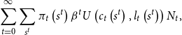 \begin{equation} \sum _{t=0}^{\infty } \sum _{s^t} \pi _t\left(s^t\right) \beta ^t U\left(c_t\left(s^t\right), l_t\left(s^t\right)\right) N_t, \end{equation}
subject to the budget constraint:
 \begin{equation*} c_t\left(s^t\right) + \left(1+\tau _{xt}\left(s^t\right)\right) x_t\left(s^t\right) = \left(1- \tau _{lt}\left(s^t\right)\right) w_t\left(s^t\right) l_t\left(s^t\right) + r_t\left(s^t\right) k_t\left(s^t\right) + T_t\left(s^t\right). \end{equation*}
where
 $\beta$
is the discount rate,
$\beta$
is the discount rate,
 $U(.)$
represents the utility function,
$U(.)$
represents the utility function,
 $N_t$
is the population (which has a growth rate of
$N_t$
is the population (which has a growth rate of
 $\gamma _n$
);
$\gamma _n$
);
 $1/(1+\tau _{x,t})$
is the investment wedge,
$1/(1+\tau _{x,t})$
is the investment wedge,
 $x_t$
is the per capita investment, (
$x_t$
is the per capita investment, (
 $1-\tau _{l,t}$
) is the labor wedge,
$1-\tau _{l,t}$
) is the labor wedge,
 $w_t$
is the real wage rate,
$w_t$
is the real wage rate,
 $r_t$
is the return on capital,
$r_t$
is the return on capital,
 $T_t$
is per capita lump-sum transfers from the government to households, and
$T_t$
is per capita lump-sum transfers from the government to households, and
 $k_t$
is the capital stock, which bears adjustment costs
$k_t$
is the capital stock, which bears adjustment costs
 $\phi\!\left(\frac{x_t\left(s^t\right)}{k_t\left(s^{t-1}\right)}\right) = \frac{a}{2}\left(\frac{x_t\left(s^t\right)}{k_t\left(s^{t-1}\right)}-b\right)^2$
, with
$\phi\!\left(\frac{x_t\left(s^t\right)}{k_t\left(s^{t-1}\right)}\right) = \frac{a}{2}\left(\frac{x_t\left(s^t\right)}{k_t\left(s^{t-1}\right)}-b\right)^2$
, with
 $b = \delta + \gamma _A + \gamma _n$
, and has the following law of accumulation:
$b = \delta + \gamma _A + \gamma _n$
, and has the following law of accumulation:
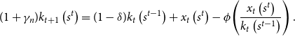 \begin{equation} (1+ \gamma _n) k_{t+1}\left(s^t\right) = (1-\delta ) k_t\left(s^{t-1}\right) + x_t\left(s^t\right) - \phi\!\left(\frac{x_t\left(s^t\right)}{k_t\left(s^{t-1}\right)}\right). \end{equation}
where
 $\delta$
is the depreciation rate.
$\delta$
is the depreciation rate.
2.1.2. Firms
The final good is produced under perfect competition and firms combine capital and labor in order to maximize profits
 $\Pi _t$
, given the production technology
$\Pi _t$
, given the production technology
 $F(k_t\left(s^{t-1}\right), (1+\gamma )^t l_t\left(s^t\right))$
:
$F(k_t\left(s^{t-1}\right), (1+\gamma )^t l_t\left(s^t\right))$
:
 \begin{equation} \max _{k_t, l_t} \Pi _t\left(s^t\right) = y_t\left(s^t\right) - r_t\left(s^t\right) k_t\left(s^{t-1}\right) - w_t\left(s^t\right) l_t\left(s^t\right) \end{equation}
Combining the first-order conditions for the household’s and firm’s maximization problems, the production function, and the resource constraint, we have the four equilibrium conditions of the model:
 \begin{equation} y_t\left(s^t\right) = A_t\left(s^t\right) F(k_t\left(s^{t-1}\right), (1+\gamma )^t l_t\left(s^t\right)) \end{equation}
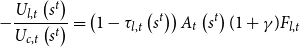 \begin{equation} -\frac{U_{l,t}\left(s^t\right)}{U_{c,t}\left(s^t\right)} = \left(1-\tau _{l,t}\left(s^t\right)\right)A_t\left(s^t\right) (1+\gamma ) F_{l,t} \end{equation}
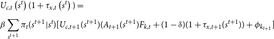 \begin{equation} \begin{aligned} & U_{c,t}\left(s^t\right) (1+\tau _{x, t}\left(s^t\right)) = \\[5pt] &\beta \sum _{s^{t+1}} \pi _t(s^{t+1}|s^t) [U_{c,t+1}(s^{t+1}) (A_{t+1}(s^{t+1}) F_{k,t} + (1-\delta )(1+\tau _{x, t+1}(s^{t+1})) + \phi _{k_{t+1}}] \end{aligned} \end{equation}
 \begin{equation} c_t\left(s^t\right) + x_t\left(s^t\right) + g_t\left(s^t\right) = y_t\left(s^t\right) \end{equation}
where
 $g_t$
is the government consumption wedge, which is assumed to fluctuate around a deterministic trend,
$g_t$
is the government consumption wedge, which is assumed to fluctuate around a deterministic trend,
 $(1 + \gamma _A)^t$
;
$(1 + \gamma _A)^t$
;
 $\gamma _A$
is the rate of labor-augmenting technical progress and
$\gamma _A$
is the rate of labor-augmenting technical progress and
 $A_t\left(s^t\right)$
is the efficiency wedge; furthermore,
$A_t\left(s^t\right)$
is the efficiency wedge; furthermore,
 $U_{c,t}$
,
$U_{c,t}$
,
 $U_{l,t}$
,
$U_{l,t}$
,
 $F_{l,t}$
,
$F_{l,t}$
,
 $F_{k,t},$
and
$F_{k,t},$
and
 $\phi _{k_{t+1}}$
represent derivatives of the utility function with respect to
$\phi _{k_{t+1}}$
represent derivatives of the utility function with respect to
 $c$
and
$c$
and
 $l$
, the derivatives of the production function with respect to
$l$
, the derivatives of the production function with respect to
 $l$
and
$l$
and
 $k$
, and the derivative of the adjustment costs function with to
$k$
, and the derivative of the adjustment costs function with to
 $k$
, respectively.
$k$
, respectively.
2.1.3. Data and calibration
We follow Chari et al. (Reference Chari, Kehoe and McGrattan2007); Brinca et al. (Reference Brinca, Chari, Kehoe and McGrattan2016) and assume the following functional forms for the utility function and the production function:
 $U(c_t\left(s^t\right), l_t\left(s^t\right))=\ln c_t+\psi _l \log (1-l_t)$
and
$U(c_t\left(s^t\right), l_t\left(s^t\right))=\ln c_t+\psi _l \log (1-l_t)$
and
 $F(k_t, l_t)= k^\alpha _t l^{1-\alpha }_t$
. The time allocation parameter
$F(k_t, l_t)= k^\alpha _t l^{1-\alpha }_t$
. The time allocation parameter
 $\psi _l$
is equal to 2.24; the capital share,
$\psi _l$
is equal to 2.24; the capital share,
 $\alpha$
, is equal to 0.35; and the discount factor
$\alpha$
, is equal to 0.35; and the discount factor
 $\beta,$
is equal to 0.9930. We also set
$\beta,$
is equal to 0.9930. We also set
 $\delta =0.0118$
and estimated
$\delta =0.0118$
and estimated
 $\gamma _n=0.0037$
from population data, and
$\gamma _n=0.0037$
from population data, and
 $\gamma _A = 0.0040$
is the rate consistent with the mean deviation of per working-age population output being equal to zero in the data. We assume that the wedges follow a VAR(1) process estimated via maximum likelihood.
$\gamma _A = 0.0040$
is the rate consistent with the mean deviation of per working-age population output being equal to zero in the data. We assume that the wedges follow a VAR(1) process estimated via maximum likelihood.
The data are taken from the OECD Quarterly National Accounts and Economic Outlook databases. In our BCA exercises, we use GDP, consumption, investment, and government consumption plus net exports time series divided by the working-age population (15 to 64 years). All variables are deflated using the GDP deflator and linearly detrended by the long-run growth rate of labor-augmenting technological process (
 $\gamma _A$
). We follow Brinca et al. (Reference Brinca, Chari, Kehoe and McGrattan2016) and adjust the data for consumption, investment, and GDP as follows. Assuming that decisions on the consumption of durable goods look like investment decisions, we subtract aggregate consumption and add to aggregate investment. We also imputed the flow of services and durable goods provided as a quarterly rental rate of one percent on the stock of durable goods (that follow a similar law of motion as the stock of physical capital, with an annualized depreciation rate calibrated to be 25%) into output.
$\gamma _A$
). We follow Brinca et al. (Reference Brinca, Chari, Kehoe and McGrattan2016) and adjust the data for consumption, investment, and GDP as follows. Assuming that decisions on the consumption of durable goods look like investment decisions, we subtract aggregate consumption and add to aggregate investment. We also imputed the flow of services and durable goods provided as a quarterly rental rate of one percent on the stock of durable goods (that follow a similar law of motion as the stock of physical capital, with an annualized depreciation rate calibrated to be 25%) into output.
Finally, we subtract sales tax revenues from both consumption and GDP. Since both sales tax data and population data are annual, we interpolate both subject to the constraint that the quarterly average of the estimated series must be equal to the annual observed data using the Denton-Cholette method (Denton, Reference Denton1971; Dagum and Cholette, Reference Dagum and Cholette2006).
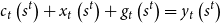
What happens with macroeconomic variables in Mexico during a crisis episode? It depends on the crisis. For instance, if we compare the dynamics of output during the 1995 crisis, the Great Recession, and the COVID crisis in Mexico, in a twelve-quarter window (ranging from the quarter after the beginning of the crisis until ten quarters after its start), we can see in the first panel of Figure 1 that output falls more rapidly and deeply and also recovers faster during the COVID crisis than in the previous episodes (considering only the same length; more data will be needed to see if the full recovery will end up being faster than the initial three quarters suggest) and is more rapidly than in the previous episodes. When comparing the 1995 crisis with the 2008 crisis, after ten quarters from the start of the crisis, output was almost fully recovered in the former, whereas it was more than 5% below its initial level in the latter.
If we take the dynamics of hours work, the recovery was also faster in the 1995 crisis (after six quarters it has achieved its initial level) rather than during the Great Recession, whereas it resembles the dynamics of output for the COVID crisis. Interestingly, the relative intensity and speed of recovery change when we consider the dynamics of investment. Not only did investment fall more rapidly during the 1995 crisis, and even during the COVID crisis, but it also took longer to recover, even though after ten quarters of the episode the level of per working-age investment was similar in the 1995 and 2008 crises.
Finally, the dynamics of government consumption plus net exports also differed between episodes. In the 1995 crisis, it rose strongly after the shock and remained at a level more than 64% higher ten quarters after the beginning of the crisis. During the Great Recession, however, it fell and recovered after three quarters, achieving a level 18% higher ten quarters afterward. When we consider the intensity and velocity of the fall in government consumption plus net exports, the COVID crisis registered the largest values, with a 22% fall during the first quarter after the shock, but in the second quarter after the crisis began, it was almost 48% higher than its initial level.
With such different observed dynamics in the four macroeconomic variables among the different crisis episodes as presented before, is it possible to identify a common mechanism? The accounting results in the next section can shed some light on the matter.
2.2. Accounting results
What are the dynamics of the four wedges in each crisis? Using the neoclassical growth model presented in Section 2.1, we estimated the path for each wedge during the three different crises. As can be seen in Figure 2, the efficiency wedge (
 $A_t$
) fell in all three recessions. However, during the 1995 and 2008 crises, the fall was much larger relative to the one during the COVID crisis. For the
$A_t$
) fell in all three recessions. However, during the 1995 and 2008 crises, the fall was much larger relative to the one during the COVID crisis. For the
 $\tau _{l,t}$
, the distortion that resembles a labor income tax, the result is the opposite, however. During the COVID crisis, it fell more than during the previous episodes. This seems to be directly related to the dynamics of hours of work in Figure 1.
$\tau _{l,t}$
, the distortion that resembles a labor income tax, the result is the opposite, however. During the COVID crisis, it fell more than during the previous episodes. This seems to be directly related to the dynamics of hours of work in Figure 1.
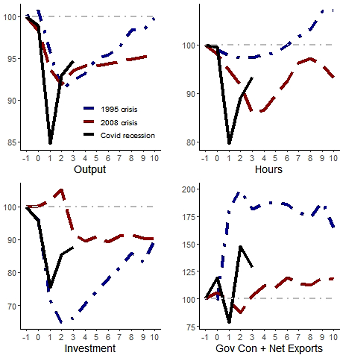
Figure 1. Macroeconomic variables during crises in Mexico. Notes: The blue curves are for the 1995 crisis, where 1994Q3 = 100; the red curves stand for the 2008 crisis with 2008Q3 = 100, and the black curves for the COVID recession, with 2019Q4 = 100. The horizontal axes present quarters relative to the beginning of the episode. All variables are divided per working-age population and with the adjustments described in the text.
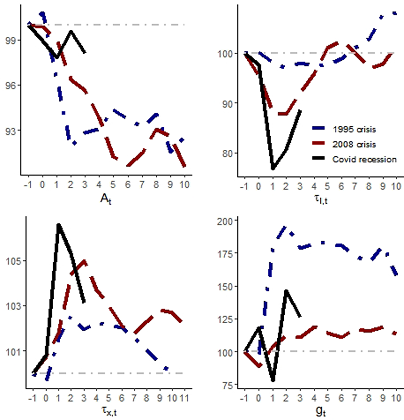
Figure 2. The behavior of estimated distortions in the model during the crises. Notes: The blue curves are for the 1995 crisis, where 1994Q3 = 100; the red curves stand for the 2008 crisis with 2008Q3 = 100, and the black curves for the COVID recession, with 2019Q4. The horizontal axes present quarters relative to the beginning of the episode.
It is worth noting that the distortion on intertemporal decisions,
 $\tau _{x,t}$
, also had a larger change during the COVID crisis, followed by the 2008 crisis, relative to the 1995 crisis, as presented in the left-handed panel side in the bottom of Figure 2. This helps to explain why investment behaved so differently during these crises, as illustrated in Figure 1. Finally, the government consumption wedge (
$\tau _{x,t}$
, also had a larger change during the COVID crisis, followed by the 2008 crisis, relative to the 1995 crisis, as presented in the left-handed panel side in the bottom of Figure 2. This helps to explain why investment behaved so differently during these crises, as illustrated in Figure 1. Finally, the government consumption wedge (
 $g_t$
) also presents very different behaviors among crises. In the next section, we decompose the wedge to understand better what is behind those differences.
$g_t$
) also presents very different behaviors among crises. In the next section, we decompose the wedge to understand better what is behind those differences.
What is the relative importance of each wedge in order to explain the dynamics of output in those episodes? After measuring/estimating the distortions, it is possible to simulate the paths of the variables in the model to see which wedge helps to account for data movements. Following Chari et al. (Reference Chari, Kehoe and McGrattan2007), the marginal effects of each wedge are obtained by keeping all other wedges fixed at their steady-state values, but the one we are interested in, for example, if we want to see the contribution of the efficiency wedge, we let it to fluctuate, while the others (labor, investment, and government consumption) are held fixed. Then, we can see how much of the data behavior the model with only one distortion can account for. The procedure also works by letting two or three wedges vary simultaneously throughout time.
The simulations with only one wedge and with only one wedge off (with only one wedge remaining constant) and the observed output paths for the 1995 and 2008 crises are presented in Figures 3 and 4.Footnote
2
Table 1 presents the statistics used to evaluate the BCA simulations: success ratio, root-mean-square error (RMSE), and the
 $\phi$
-statistic presented in Brinca et al. (Reference Brinca, Chari, Kehoe and McGrattan2016):
$\phi$
-statistic presented in Brinca et al. (Reference Brinca, Chari, Kehoe and McGrattan2016):
 \begin{equation*} \phi ^y_i = \frac {1/\sum _t (y^D_t-y_{i,t})^2}{\sum _{j} (1/\sum _t (y^D_t-y_{i,t})^2)}, \end{equation*}
where
 $y^D_t$
is the observed data for output,
$y^D_t$
is the observed data for output,
 $y_{i,t}$
is the simulated path for output prescribed by model
$y_{i,t}$
is the simulated path for output prescribed by model
 $i \in [1, j]$
. The statistics lie between
$i \in [1, j]$
. The statistics lie between
 $0$
and
$0$
and
 $1$
, and the closer the value is to
$1$
, and the closer the value is to
 $1$
, more it accounts for observed movements in the data.
$1$
, more it accounts for observed movements in the data.
Figure 3. Simulated output trajectory during the 1995 crisis. Notes: The red curves are for the model with (without) the efficiency wedge in one-wedge (off) economies; analogously, the green curves are related to the labor wedge, the blue curves to the investment wedge, and the orange curves to the government consumption wedge. The black line is the observed data. 1994Q4 = 100.
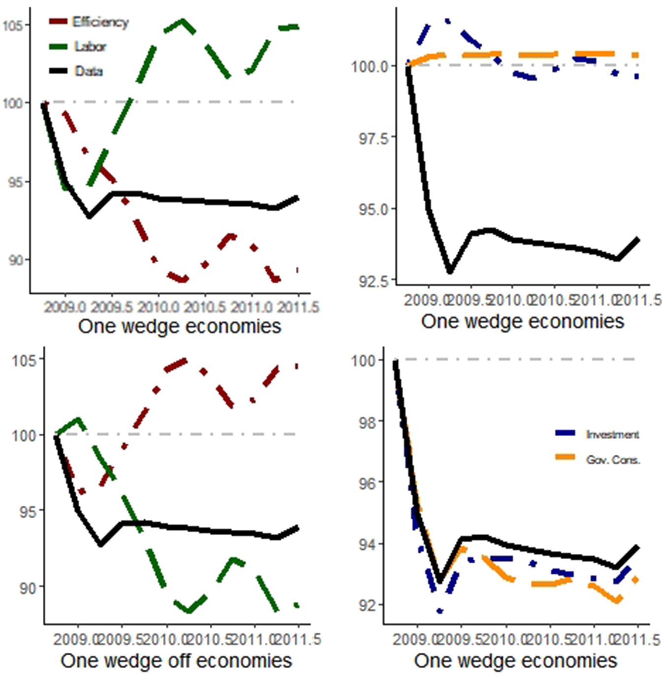
Figure 4. Simulated output trajectory during the 2008 crisis. Notes: The red curves are for the model with (without) the efficiency wedge in one-wedge (off) economies; analogously, the green curves are related to the labor wedge, the blue curves to the investment wedge, and the orange curves to the government consumption wedge. The black line is the observed data. 1994Q4 = 100.
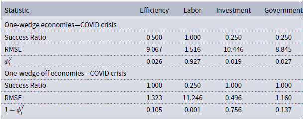
Table 1. BCA decomposition statistics
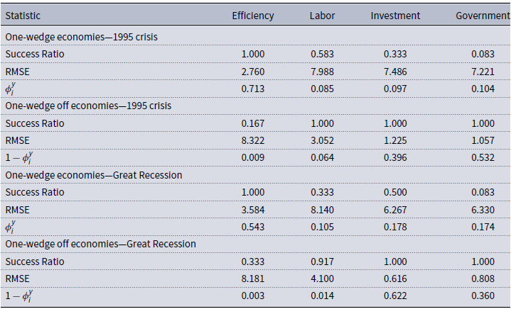
Success ratio: the relative frequency when simulated and observed data had the same sign; linear correlations between simulated and observed data; RMSE: root of the mean-square error;
 $\phi$
-statistic following Brinca et al. (Reference Brinca, Chari, Kehoe and McGrattan2016). For the two crises, we consider a 12-quarter window; we define the first quarters of the BCA exercise as 1994Q4 and 2008Q2.
$\phi$
-statistic following Brinca et al. (Reference Brinca, Chari, Kehoe and McGrattan2016). For the two crises, we consider a 12-quarter window; we define the first quarters of the BCA exercise as 1994Q4 and 2008Q2.
The efficiency wedge alone has the best performance among one-wedge economies for both episodes. The model with only that distortion accounts for 71.3% of whole output movements during the 1995 crisis and 54.3% during the Great Recession. The investment and government consumption wedges explain around 10% of GDP fluctuations during the 1995 crisis, while their relative contributions rise to around 17% during the Great Recession.
The poor performance of the models with only government consumption raises a question. Given that the 1995 episode was a currency crisis (followed by a large increase in net exports) and that the 2008 episode was an international crisis, shouldn’t they both be transmitted through the balance of payments and/or assigning a greater role to the government consumption wedge due to an increase in net exports following exchange rate depreciation? This calls for a further investigation of the dynamics of the government consumption wedge. In Figure 5, we have decomposed the dynamics of the government consumption wedge into the changes in government consumption, exports, and imports for the 1995 and 2008 crises.
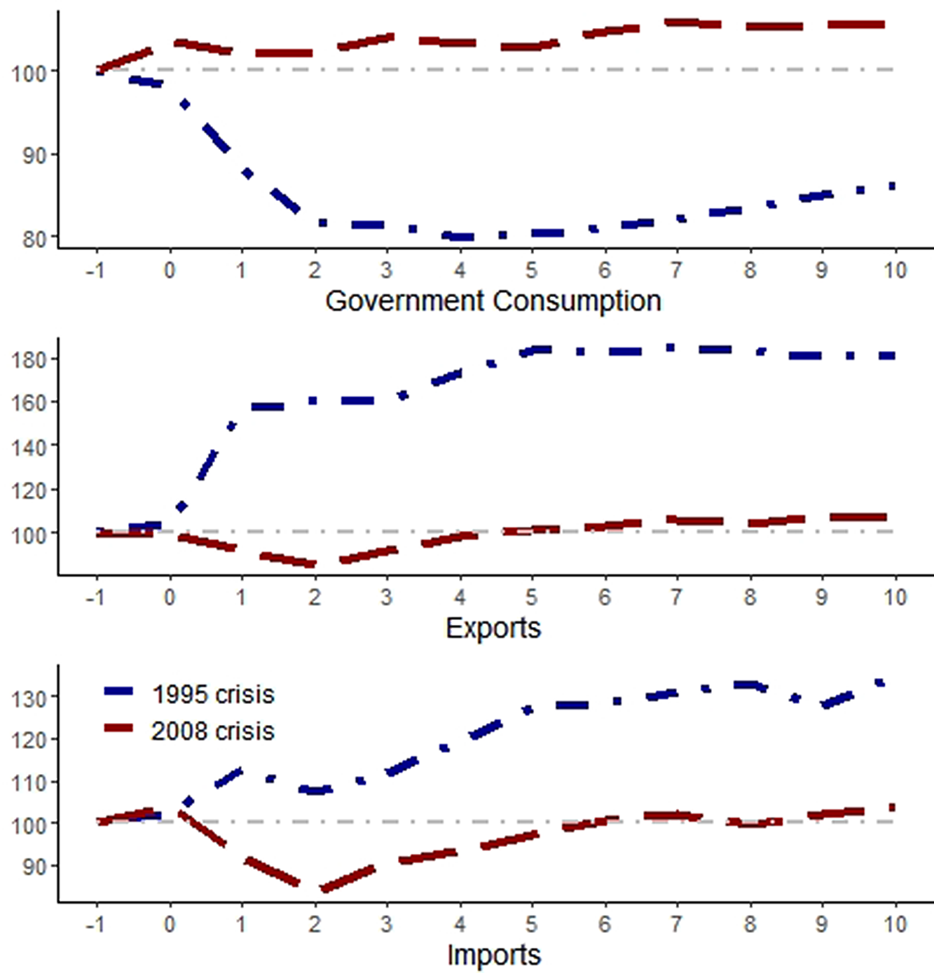
Figure 5. Decomposition of the government consumption wedge for the 1995 and 2008 crises. Notes: The blue curves are for the 1995 crisis, where 1994Q3 = 100; the red curves stand for the 2008 crisis with 2008Q3 = 100, and the black curves for the COVID recession, with 2019Q4. The horizontal axes present quarters relative to the beginning of the episode.
We can see in the top panel of Figure 5 that the fiscal response was very different between crises. In 1995, the decrease in government spending offset the increase in net exports (see that exports in the middle panel rose more than imports in the bottom panel). In 2008, however, there was an increase in both government spending and net exports. This probably helps to explain why the relative role of the government consumption wedge rises from around 10% to more than 17%.
Given the prominent role of the efficiency wedge in explaining a large share of output fluctuations in both crises, we explore in the next section what is behind the efficiency wedge and how it is related to output falls and the international transmission of crises.
3. Structural interpretation of the wedges
After being informed by the BCA exercises that the efficiency wedge is the main driver of output during both crises, we need to understand how output could be affected in Mexico via distortions in the production side of the economy. Since 1990, the Mexican economy has become increasingly reliant on imported intermediate goods, as illustrated in Figure 6. For the sake of comparison, we see that the share of foreign intermediate goods in the GDP is much higher in Mexico than in the USA.
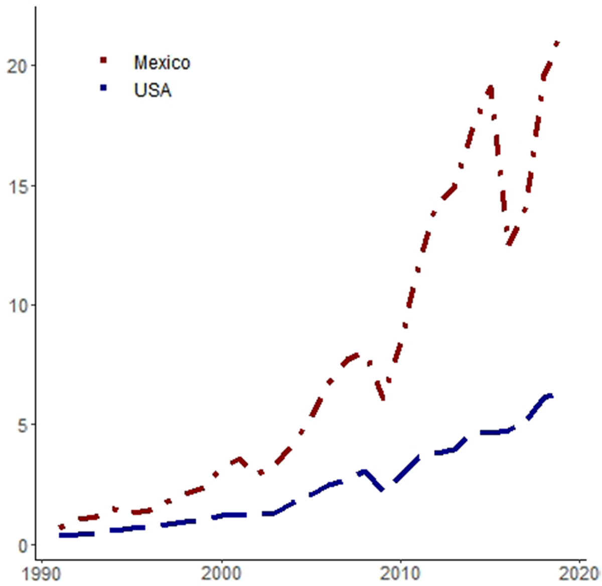
Figure 6. Intermediate goods imports share of GDP (%). Notes: The red curves represents data for Mexico and the blue curve is the data for the USA. See the appendix for the data details.
The Mexican economy was hit by at least two shocks during the Great Recession: falling exports due to lower demand from the USA and a risk-aversion movement that depreciated the exchange rate (Sidaoui et al. Reference Sidaoui, Ramos-Francia and Cuadra2010). The combination of shocks made foreign intermediate inputs more expensive and was associated with a fall in output at the same time. We can see in Figure 7 that the log-detrended per capita output and the deviations from the purchase power parity equilibrium for the real exchange rate are negatively correlated (the coefficient of linear correlation for both series is −0.54 in our sample).
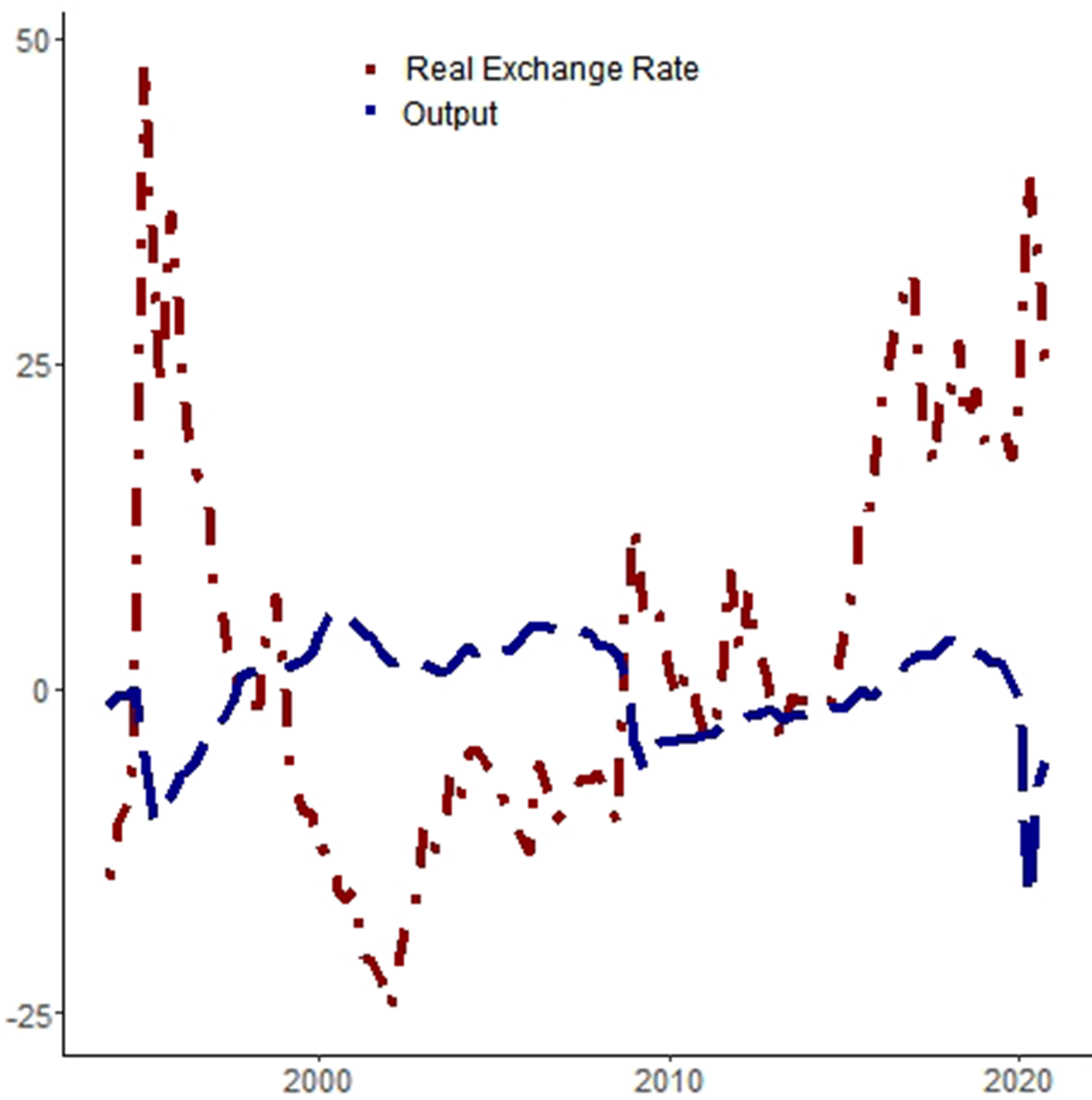
Figure 7. Output and real exchange rate changes (%). Notes: The red line stands for deviations from the long-run real exchange rate, which should be equal to 1 according to the purchase power parity theory; the blue line is log-detrended per working-age person output. A rise in the exchange rate means depreciation.
With all that in mind, the next section presents a model with imported goods in the production function to understand the dynamics of output during the 1995 and 2008 crises in Mexico and how an efficiency wedge may arise from the imports of intermediate goods.Footnote 3
3.1. Detailed economy
We introduce imported intermediate inputs in the final goods production in Schmitt-Grohé and Uribe (Reference Schmitt-Grohé and Uribe2003) small open-economy debt-elastic interest rate model. Households behave in a rational way and derive utility from consumption (
 $c_t$
) and disutility from hours worked (
$c_t$
) and disutility from hours worked (
 $l_t$
). As is usual in this kind of model, households have a positive but decreasing marginal utility of consumption and an increasing marginal disutility of labor. The domestic agents can use their own resources as well as foreign capital. The dynamics of foreign debt (
$l_t$
). As is usual in this kind of model, households have a positive but decreasing marginal utility of consumption and an increasing marginal disutility of labor. The domestic agents can use their own resources as well as foreign capital. The dynamics of foreign debt (
 $d_t$
) are given by:
$d_t$
) are given by:
 \begin{equation} d_t = (1 + r_{t-1}) d_{t-1} - q_t + c_t + x_t + e_t m_t. \end{equation}
where
 $d_t$
is the foreign debt,
$d_t$
is the foreign debt,
 $r_t$
is the one-period real interest rate,
$r_t$
is the one-period real interest rate,
 $q_t$
stands for gross output,
$q_t$
stands for gross output,
 $x_t$
represents investment,
$x_t$
represents investment,
 $m_t$
stands for imported intermediate goods, and
$m_t$
stands for imported intermediate goods, and
 $e_t$
is the foreign (imported intermediate goods) prices over domestic prices. The interest rate is a function of the equilibrium interest rate and the country’s foreign indebtedness level.
$e_t$
is the foreign (imported intermediate goods) prices over domestic prices. The interest rate is a function of the equilibrium interest rate and the country’s foreign indebtedness level.
 $r_t = r + \psi (\! \exp(d_t-d) -1)$
, where
$r_t = r + \psi (\! \exp(d_t-d) -1)$
, where
 $r$
represents the steady-state real interest rate,
$r$
represents the steady-state real interest rate,
 $d$
represents the equilibrium value of foreign debt, and
$d$
represents the equilibrium value of foreign debt, and
 $\psi$
is a parameter.
$\psi$
is a parameter.
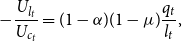
Gross output is produced by combining imported intermediate goods, capital, and labor as follows:
 \begin{equation} q_t = m^{\mu }_t (k^{\alpha }_t l^{1-\alpha }_t)^{1-\mu }. \end{equation}
where
 $k$
is the stock of productive capital, which has a share of
$k$
is the stock of productive capital, which has a share of
 $\alpha$
in total output, and
$\alpha$
in total output, and
 $\mu$
is the share of imported intermediate goods.
$\mu$
is the share of imported intermediate goods.
We assume
 $e_t$
to be exogenous, following an AR(1) process:
$e_t$
to be exogenous, following an AR(1) process:
 \begin{equation} \ln e_t = ( 1 - \rho _e) \ln e + \rho _e \ln e_{t-1} + \epsilon ^{e}_t. \end{equation}
where
 $\rho _e$
is the persistence parameter,
$\rho _e$
is the persistence parameter,
 $e$
without the subscript
$e$
without the subscript
 $t$
is the steady-state value of
$t$
is the steady-state value of
 $e_t$
, and
$e_t$
, and
 $\epsilon ^{e}_t$
is a shock. The law for capital accumulation is given by:
$\epsilon ^{e}_t$
is a shock. The law for capital accumulation is given by:
 \begin{equation} k_{t+1} = (1-\delta ) k_t + x_t - \Lambda (k_{t+1}). \end{equation}
where
 $\Lambda (k_{t+1}) = \frac{\eta }{2}(k_{t+1} - k_t)^2$
represents capital adjustment costs.
$\Lambda (k_{t+1}) = \frac{\eta }{2}(k_{t+1} - k_t)^2$
represents capital adjustment costs.
Under the presented assumptions, the optimization problem is given by:
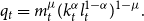
 \begin{equation} \max _{c_t, l_t, d_t, k_{t+1}} E_t \sum _{t=0}^{\infty } \beta ^t U(c_t, l_t) \end{equation}
where
 $U(c_t, l_t)$
is the instantaneous utility, subject to the debt dynamics from equation 8, the production technology expressed in equation 9, the law for capital accumulation (equation 11), taking the exogenous movements of the real exchange rate (equation 10) and the real interest rate as given.
$U(c_t, l_t)$
is the instantaneous utility, subject to the debt dynamics from equation 8, the production technology expressed in equation 9, the law for capital accumulation (equation 11), taking the exogenous movements of the real exchange rate (equation 10) and the real interest rate as given.
One more restriction should be imposed to assure non-Ponzi dynamics in the system. The transversality condition is given by:
 \begin{equation} \lim \limits _{j \rightarrow \infty } E_t \frac{d_{t+j}}{\prod ^{j}_{s} (1+r_{s})} \leq 0, \end{equation}
which implies that the present value of the debt should be less than or equal to zero, that is, there should be no remaining debt at the limit.
The first-order conditions with respect to
 $d_{t+1}, c_t, l_t, k_{t+1}$
and
$d_{t+1}, c_t, l_t, k_{t+1}$
and
 $m_t$
are as follows:
$m_t$
are as follows:
 \begin{equation} \lambda _t = \beta E_t \lambda _{t+1} (1 + r_{t}), \end{equation}
 \begin{equation} \lambda _t = U_{c_{t}}, \end{equation}
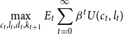
 \begin{equation} -\frac{U_{l_{t}}}{U_{c_{t}}} = (1-\alpha ) (1-\mu ) \frac{q_t}{l_t}, \end{equation}
 \begin{equation} \lambda _t (1+ \phi (k_{t+1} - k_t)) = \beta E_t \lambda _{t+1} \big(\eta (k_{t+2} - k_{t+1}) + 1-\delta + (1-\mu ) \alpha \frac{q_{t+1}}{k_{t+1}} \big), \end{equation}
 \begin{equation} \frac{\mu q_t}{m_t} = e_t, \end{equation}
where
 $\partial U(c_t, l_t)/\partial c_t = U_{c_{t}}$
and
$\partial U(c_t, l_t)/\partial c_t = U_{c_{t}}$
and
 $\partial U(c_t, l_t)/\partial l_t = U_{l_{t}}$
and
$\partial U(c_t, l_t)/\partial l_t = U_{l_{t}}$
and
 $\lambda _t$
represent the Lagrange multiplier. The definition of trade balance over GDP (
$\lambda _t$
represent the Lagrange multiplier. The definition of trade balance over GDP (
 $tby_t$
) closes the model:
$tby_t$
) closes the model:
 \begin{equation} 1 - \frac{c_t}{y_t} - \frac{x_t}{y_t} = tby_t. \end{equation}
where
 $y_t = q_t - e_t m_t$
is the value-added output. We assume that all intermediate goods produced domestically are exported.
$y_t = q_t - e_t m_t$
is the value-added output. We assume that all intermediate goods produced domestically are exported.
3.2. Shocks to relative prices as shocks to productivity: an equivalence
How does the detailed economy relate to the prototype model in Section 2.1? In Proposition 1, we can map the equilibrium allocations of the small open-economy model with imported intermediate inputs into the prototype economy used in the BCA exercises and provide a structural interpretation for the wedges (we thank the referee for his suggestions to improve the exposition of the proposition and the discussion of the results).
Proposition 1.
Consider the prototype economy previously described, with
 $A_t =(1-\mu )\left (\frac{\mu }{e_{t}}\right )^{\frac{\mu }{1-\mu }}$
,
$A_t =(1-\mu )\left (\frac{\mu }{e_{t}}\right )^{\frac{\mu }{1-\mu }}$
,
 $(1+\tau _{x,t}) = (1+ \eta (k_{t+1} - k_t))$
,
$(1+\tau _{x,t}) = (1+ \eta (k_{t+1} - k_t))$
,
 $(1+\tau _{x,t+1}) = 1+ (1+ \eta (k_{t+2} - k_{t+1}))/(1-\delta )$
,
$(1+\tau _{x,t+1}) = 1+ (1+ \eta (k_{t+2} - k_{t+1}))/(1-\delta )$
,
 $(1- \tau _{l,t}) = 0$
and
$(1- \tau _{l,t}) = 0$
and
 $g_t = (1 + r_{t-1}) d_{t-1} - d_t$
. The equilibrium allocations in the detailed economy match equilibrium allocations in the prototype economy.
$g_t = (1 + r_{t-1}) d_{t-1} - d_t$
. The equilibrium allocations in the detailed economy match equilibrium allocations in the prototype economy.
Proof. The efficiency wedge mapping is obtained by substituting the first-order condition with respect to
 $m_t$
(equation 18) for the gross production function (equation 9):
$m_t$
(equation 18) for the gross production function (equation 9):
 $q_{t}=\left (\mu \frac{q_{t}}{e_{t}}\right )^{\mu }\left (k_{t}^{\alpha } l_{t}^{1-\alpha }\right )^{1-\mu }=\left (\frac{\mu }{e_{t}}\right )^{\frac{\mu }{1-\mu }} k_{t}^{\alpha } l_{t}^{1-\alpha }$
. According to the definition of the value-added output, we have that
$q_{t}=\left (\mu \frac{q_{t}}{e_{t}}\right )^{\mu }\left (k_{t}^{\alpha } l_{t}^{1-\alpha }\right )^{1-\mu }=\left (\frac{\mu }{e_{t}}\right )^{\frac{\mu }{1-\mu }} k_{t}^{\alpha } l_{t}^{1-\alpha }$
. According to the definition of the value-added output, we have that
 $y_{t}=q_{t}-e_{t} m_{t}=(1-\mu ) q_{t}=(1-\mu )\left (\frac{\mu }{e_{t}}\right )^{\frac{\mu }{1-\mu }} k_{t}^{\alpha } l_{t}^{1-\alpha }$
, or
$y_{t}=q_{t}-e_{t} m_{t}=(1-\mu ) q_{t}=(1-\mu )\left (\frac{\mu }{e_{t}}\right )^{\frac{\mu }{1-\mu }} k_{t}^{\alpha } l_{t}^{1-\alpha }$
, or
 $y_{t}=A_t k_{t}^{\alpha } l_{t}^{1-\alpha }$
, where
$y_{t}=A_t k_{t}^{\alpha } l_{t}^{1-\alpha }$
, where
 $A_t =(1-\mu )\left (\frac{\mu }{e_{t}}\right )^{\frac{\mu }{1-\mu }}$
. The labor wedge distorts the intratemporal decision. In the detailed economy, there is no such distortion. It is easy to see that if we compare equation 16 with equation 5 using the definition of GDP,
$A_t =(1-\mu )\left (\frac{\mu }{e_{t}}\right )^{\frac{\mu }{1-\mu }}$
. The labor wedge distorts the intratemporal decision. In the detailed economy, there is no such distortion. It is easy to see that if we compare equation 16 with equation 5 using the definition of GDP,
 $y_{t} = (1-\mu ) q_{t};$
thus,
$y_{t} = (1-\mu ) q_{t};$
thus,
 $(1- \tau _{l,t}) = 0$
. From equation 15, we have the marginal utility of consumption. The right-hand side of equation 6 presents the marginal utility of consumption, which is equal to the Lagrange multiplier, times the inverse of the investment wedge. By equating the left-hand side of equation 17 to the left-hand side of equation 6, we have that
$(1- \tau _{l,t}) = 0$
. From equation 15, we have the marginal utility of consumption. The right-hand side of equation 6 presents the marginal utility of consumption, which is equal to the Lagrange multiplier, times the inverse of the investment wedge. By equating the left-hand side of equation 17 to the left-hand side of equation 6, we have that
 $(1+\tau _{x,t}) = (1+ \eta (k_{t+1} - k_t))$
. Moreover, making the right-hand sides of the two equations equal yields
$(1+\tau _{x,t}) = (1+ \eta (k_{t+1} - k_t))$
. Moreover, making the right-hand sides of the two equations equal yields
 $\beta E_t[u_{c,t+1} (A_{t+1} F_{kt} + (1-\delta )(1+\tau _{x, t+1}))] = \beta E_t \lambda _{t+1} (\eta (k_{t+2} - k_{t+1}) + 1-\delta + (1-\mu ) \alpha \frac{y_{t+1}}{k_{t+1}}) \iff (1+\tau _{x,t+1}) = 1+ (1+ \eta (k_{t+2} - k_{t+1}))/(1-\delta )$
. Finally, the government consumption wedge can be calculated directly from the trade balance (equation 8 and equation 19):
$\beta E_t[u_{c,t+1} (A_{t+1} F_{kt} + (1-\delta )(1+\tau _{x, t+1}))] = \beta E_t \lambda _{t+1} (\eta (k_{t+2} - k_{t+1}) + 1-\delta + (1-\mu ) \alpha \frac{y_{t+1}}{k_{t+1}}) \iff (1+\tau _{x,t+1}) = 1+ (1+ \eta (k_{t+2} - k_{t+1}))/(1-\delta )$
. Finally, the government consumption wedge can be calculated directly from the trade balance (equation 8 and equation 19):
 $y_t - x_t - c_t = g_t = (1 + r_{t-1}) d_t - d_t$
.
$y_t - x_t - c_t = g_t = (1 + r_{t-1}) d_t - d_t$
.
We can see from the definition of the efficiency wedge in the equivalence above,
 $A_t =$
 $(1-\mu )\left (\frac{\mu }{e_{t}}\right )^{\frac{\mu }{1-\mu }}$
, that an increase in relative prices manifests itself as a deterioration in the efficiency wedge. This is a key result of this paper. By extending a simple small open-economy model with the introduction of imported intermediate goods into the gross production function, we have revealed how international shocks such as terms of trade shock and/or a nominal exchange rate shock have real effects on GDP. For instance, an increase in foreign prices relative to domestic prices produces a negative impact on production that is not matched by a proportional decrease in imports, since capital and labor are not perfect substitutes and, at least in the short run, domestic firms cannot replace the imported intermediate goods. Proposition 1 offers a solution to the puzzle presented by Kehoe and Ruhl (Reference Kehoe and Ruhl2008). Furthermore, it reveals a “missing” international link as a mechanism for the transmission of crises in the efficiency wedge and why the government consumption wedge played a smaller role in explaining output fluctuations during the 1995 and 2008 crises.
$(1-\mu )\left (\frac{\mu }{e_{t}}\right )^{\frac{\mu }{1-\mu }}$
, that an increase in relative prices manifests itself as a deterioration in the efficiency wedge. This is a key result of this paper. By extending a simple small open-economy model with the introduction of imported intermediate goods into the gross production function, we have revealed how international shocks such as terms of trade shock and/or a nominal exchange rate shock have real effects on GDP. For instance, an increase in foreign prices relative to domestic prices produces a negative impact on production that is not matched by a proportional decrease in imports, since capital and labor are not perfect substitutes and, at least in the short run, domestic firms cannot replace the imported intermediate goods. Proposition 1 offers a solution to the puzzle presented by Kehoe and Ruhl (Reference Kehoe and Ruhl2008). Furthermore, it reveals a “missing” international link as a mechanism for the transmission of crises in the efficiency wedge and why the government consumption wedge played a smaller role in explaining output fluctuations during the 1995 and 2008 crises.
3.3. Quantitative exercise
In Section 3.1, we presented the structural model for understanding the main drivers of output during the 1995 and 2008 crises. In Section 3.2, we showed that relative price shocks generate changes in the efficiency wedge in the model, and we know from the results of Section 2.2 this is the main distortion that we need in the neoclassical growth model to account for observed GDP fluctuations. How does the model capture the dynamics of output during both crises, namely the largest fall and faster recovery in the 1995 crisis relative to the 2008 episode?
In order to answer that question, we perform a stochastic simulation of the log-linearized version of the model with a sequence of shocks on the relative prices as the deviations from the steady state and compare the prescribed path for GDP growth with the observed deviations of output from its estimated trend during two windows: 1994Q1–1997Q2 and 2008Q3–2015Q1.
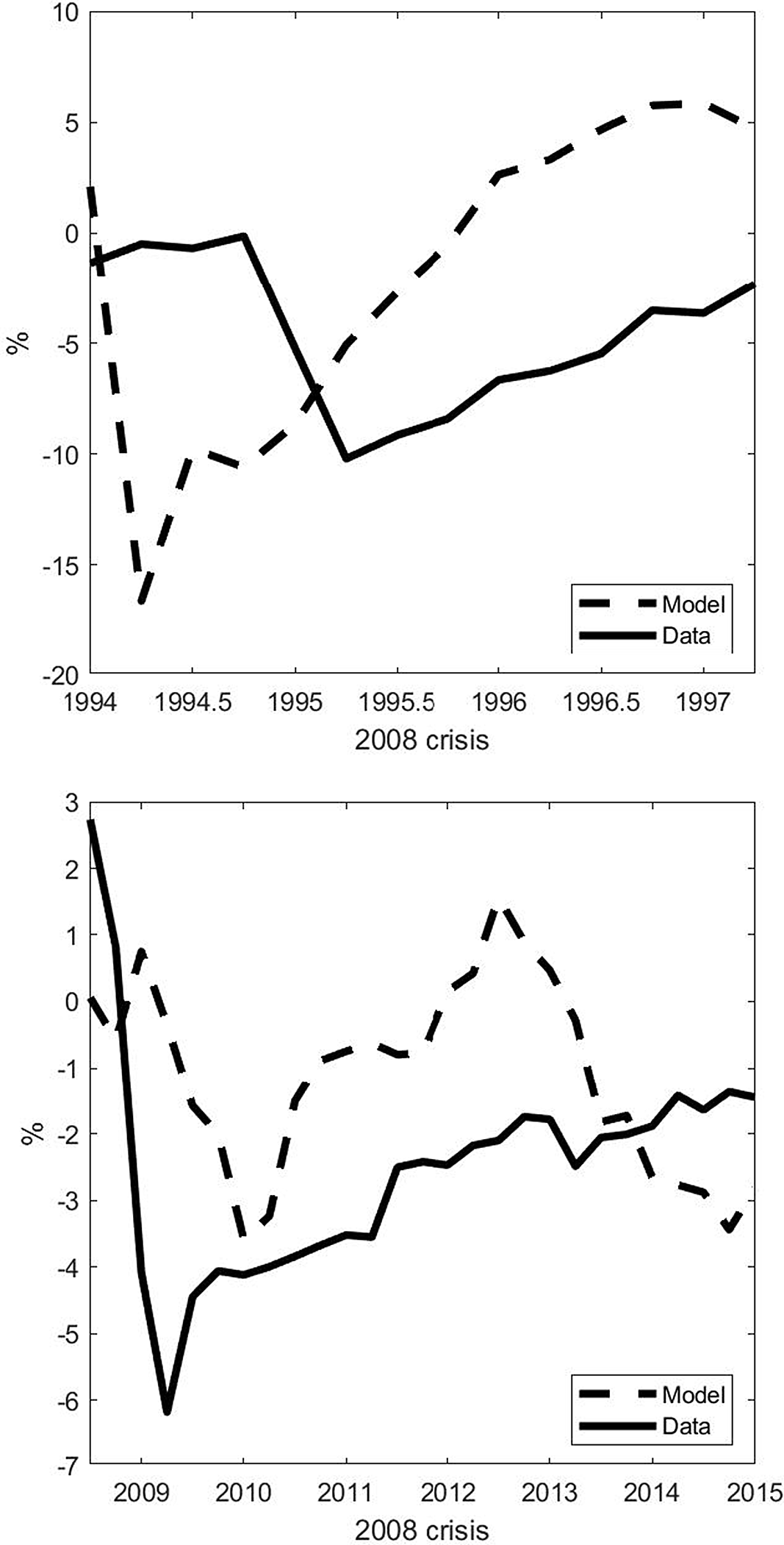
Figure 8. The dynamics of output during the 1995 and the 2008 crises: data vs simulations. Notes: In both graphs, the solid line stands for log-detrended data on output, and the dashed line refers to the simulation of the log-linearized version of the detailed economy with the exogenous shocks on the real exchange rate. On the top panel, the simulation is for the 1994Q1–1997Q2 period. On the bottom panel, the simulation is for the 2008Q3–2015Q1 period.
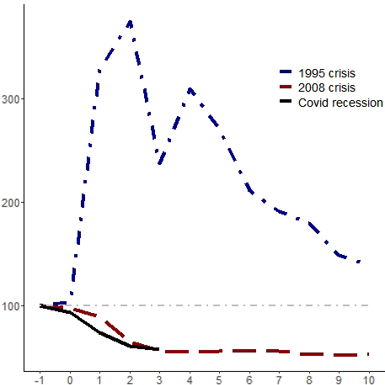
Figure 9. Short-run interest rate during the three crises in Mexico. Notes: The blue curves are for the 1995 crisis, where 1994Q3 = 100; the red curves stand for the 2008 crisis, with 2008Q3 = 100, and the black curves are for the COVID recession, with 2019Q4. The horizontal axes present quarters relative to the beginning of the episode.
3.3.1. Data, calibration, and functional form
In our quantitative exercises, we use the following function for households’ preferences:
 $U(c_t, l_t) \frac{[c_t - \omega ^{-1} l^{\omega }_t]^{1-\gamma }-1}{1-\gamma }$
. Each time period is equivalent to one quarter. On our parametrization strategy, we use the Euler equation evaluated at steady state and the 1991–2010 mean of the internal rate of return from the Penn World Table (version 10.0) to set the discount factor equal to
$U(c_t, l_t) \frac{[c_t - \omega ^{-1} l^{\omega }_t]^{1-\gamma }-1}{1-\gamma }$
. Each time period is equivalent to one quarter. On our parametrization strategy, we use the Euler equation evaluated at steady state and the 1991–2010 mean of the internal rate of return from the Penn World Table (version 10.0) to set the discount factor equal to
 $\beta =0.9665$
(we also experimented with the mean of the real interest rate from the World Development Indicators, which yields a
$\beta =0.9665$
(we also experimented with the mean of the real interest rate from the World Development Indicators, which yields a
 $\beta =0.9907$
, and the results are very similar). From the same source, we use the 1991-2010 mean of the depreciation rate, which yields a yearly depreciation rate,
$\beta =0.9907$
, and the results are very similar). From the same source, we use the 1991-2010 mean of the depreciation rate, which yields a yearly depreciation rate,
 $\delta =0.03$
, and the share of labor compensation in GDP at current national prices, leading to
$\delta =0.03$
, and the share of labor compensation in GDP at current national prices, leading to
 $\alpha = 0.61$
.
$\alpha = 0.61$
.
From the steady state, we know that
 $\mu = m/ q$
, assuming
$\mu = m/ q$
, assuming
 $e=1$
. We take the average share of imported intermediate goods relative to GDP (1991–2010) to set
$e=1$
. We take the average share of imported intermediate goods relative to GDP (1991–2010) to set
 $\mu =0.0667$
.
$\mu =0.0667$
.
 $\rho _e=0.86$
is the estimated an AR(1) coefficient with data for the relative prices, explained below with the shocks. We use the average (1993-2010) net foreign assets data from the World Development Indicators to set
$\rho _e=0.86$
is the estimated an AR(1) coefficient with data for the relative prices, explained below with the shocks. We use the average (1993-2010) net foreign assets data from the World Development Indicators to set
 $d/y = 0.0695$
. We set
$d/y = 0.0695$
. We set
 $\omega =2.1765$
to produce the same Frisch elasticity of labor supply as in Lama et al. (Reference Lama, Leyva and Urrutia2022). We take
$\omega =2.1765$
to produce the same Frisch elasticity of labor supply as in Lama et al. (Reference Lama, Leyva and Urrutia2022). We take
 $\eta =0.028$
and
$\eta =0.028$
and
 $\psi =0.000742$
(we also simulated with a very small number just to ensure convergence as in Lama et al. (Reference Lama, Leyva and Urrutia2022),
$\psi =0.000742$
(we also simulated with a very small number just to ensure convergence as in Lama et al. (Reference Lama, Leyva and Urrutia2022),
 $\psi$
=1e-8 and the results do not change) from Schmitt-Grohé and Uribe (Reference Schmitt-Grohé and Uribe2003). Finally, we set
$\psi$
=1e-8 and the results do not change) from Schmitt-Grohé and Uribe (Reference Schmitt-Grohé and Uribe2003). Finally, we set
 $\gamma = 2$
(the quantitative results almost do not change for
$\gamma = 2$
(the quantitative results almost do not change for
 $\gamma \in [1,3]$
).
$\gamma \in [1,3]$
).
3.3.2. Shocks
We have the following steps for shocks to the relative price ratio: (i) We calculated the log of the import deflator over the GDP deflator ratio from 1993Q1 to 2020Q4. We use data from the Quarterly National Accounts database (OECD). Then, (ii) we linearly detrend the time series; (iii) with the detrended data, we calculated the four-quarters moving average; and (iv) we estimate an AR(1) model with the resulting series and use the residuals as the shocks in the stochastic simulations. The data sources are presented in Section A.4 in the Appendix.
We can see in the top panel of Figure 8 that the model is able to account for the large fall and rapid recovery of GDP during the 1995 crisis. There was a large increase in foreign prices relative to domestic prices in that period, which decreased output via a fall in the efficiency wedge. Imported intermediate goods became more expensive quickly, reducing gross output even as net exports increased (see Figure 5). This finding complements the existing literature on the 1995 crisis that attributes banking fragility, changes in world capital movements, economic policy, and foreign interest rates to the roots of the crisis (Kaminsky et al. Reference Kaminsky, Reinhart and Vegh2003; Calvo and Mendoza, Reference Calvo and Mendoza1996) by adding in another driver of output fall and recovery, intermediate goods imports.
During the 2008 crisis, there was also an increase in foreign prices relative to domestic prices, but the change was considerably less intense than the one during the 1995 crisis. However, it had a sequence of depreciation and appreciation cycles that lasted longer than during the 1995 crisis episode. This is reflected in the simulated path for output in the panel on the bottom of Figure 8. The model is able to reproduce the slower recovery and a large share of the GDP fall during the crisis.
3.4. Investment and labor frictions
What are the candidates for the investment and labor wedges? For the former, we believe that shocks to the capital accumulation process, as in Cooper and Ejarque (Reference Cooper and Ejarque2000) could explain the observed path of the distortion during the aforesaid crises. The nature of the shock might differ, though. We can see in Figure 9 that the short-run interest rate rose rapidly during the 1995 balance-of-payments crisis, whereas it had the opposite movement amid the 2008 and the COVID crises. We consider this as an indication that in 1995, a shock on the country’s risk premium might have affected capital accumulation, whereas during the other two crises, the nature of the shock was more on entrepreneurs’ (and banks’) confidence and/or difficulties within a financial accelerator with nominal rigidity set up as in Gertler and Kiyotaki (Reference Gertler and Kiyotaki2010), since monetary policy was expansionary, not only via interest rates but also by alleviating credit market constraints. See Brinca et al. (Reference Brinca, Costa-Filho and Loria2020) for other sorts of detailed economies that can generate investment wedges.
Finally, for the labor wedge, we hypothesize that it can be the result of one (or a combination) of three types of frictions: financial frictions may have contributed to the labor wedge as in Mendoza (Reference Mendoza2010), as well as markups in products and labor markets as in Gali et al. (Reference Gali, Gertler and Lopez-Salido2007) and labor market policies operating in an environment with search and matching frictions with an endogenous selection mechanism that can not only influence the labor wedge but also the dynamics of aggregate productivity (Lama et al. Reference Lama, Leyva and Urrutia2022).
4. Final remarks
In this paper, we analyze the drivers of output during two major crises in Mexico: the 1995 balance-of-payments crisis and the Great Recession. We also provided an initial account of the COVID crisis. Even though they differ in the nature, intensity, and velocity of recovery, we examine whether it is possible to identify a common mechanism among them.
We used the BCA method developed by Chari et al. (Reference Chari, Kehoe and McGrattan2007) to identify and inform us about the main candidates for explaining output dynamics during the aforementioned crises. By simulating the trajectory of output with and without letting each distortion in the neoclassical growth model fluctuate, the accounting result finds that the efficiency wedge is the most relevant distortion.
We interpret the falling efficiency wedge during each crisis as a consequence of changes in foreign prices relative to domestic prices. We formalize this result in an equivalence between the prototype economy with wedges and a small open-economy model augmented with imported intermediate goods.
The equivalence suggests that the negative relationship between shocks to the real exchange rate and changes in productivity offers a solution to the puzzle presented by Kehoe and Ruhl (Reference Kehoe and Ruhl2008). They argue in their paper that trade shocks, which empirical evidence shows are negatively related to productivity, do not have first-order effects on output in the models they study. In this paper, without necessarily relying on tariff shocks or financial frictions, our model presents a framework that helps to reconcile theory and empirical evidence.
Our model is able to capture the distinct dynamics of output between the 1995 and 2008 crises, namely the observed faster recovery in the former than in the latter, with only one exogenous variable: a ratio between foreign and domestic prices.
Given the growing economic integration the world has experienced, along with the fact that the frequency of financial crises has increased, it is important to dissect any role international trade may play in transmitting the crisis from one country to another. This does not diminish the importance of other channels, but our paper has shown that accounting for relative price shocks in small open economies with imported intermediate goods requires considering the international link “hidden” within the efficiency wedge, which would have been missed by only observing the movements in net exports.
Appendix A. DATA SOURCES
A.1. BCA DATA
The data used for the BCA exercises were obtained from the OECD databases (variable codes in parentheses). The sample for quarterly data is from 1993Q1 to 2020Q4. For the working-age population, the annual data span is from 1993 to 2020.
-
• Quarterly National Accounts Database
-
Gross domestic product (B1_GE): expenditure approach, millions of national currency, current prices, quarterly levels, s.a.
-
Deflator (B1_GE): national base/reference year, s.a. (It has the same code as the previous variable, what changes are the “measure” in the database).
-
Private final consumption expenditure (P31S14_S15): millions of national currency, current prices, quarterly levels, s.a.
-
Final consumption expenditure of general government (P3S13): millions of national currency, current prices, quarterly levels, s.a.
-
Gross capital formation (P5): millions of national currency, current prices, quarterly levels, s.a.
-
Exports of goods and services (P6): Millions of national currency, current prices, quarterly levels, s.a.
-
Imports of goods and services (P7): Millions of national currency, current prices, quarterly levels, s.a.
-
• Economic Outlook No 110—December 2021 database
-
Hours worked: per worker, total economy.
-
Total employment (ET): national accounts basis.
-
• Historical Population Database
-
Population: Total (T), Working-age population: 15 to 64 years old (15–64).
Data transformation: population data are available at an annual frequency and are interpolated to a quarterly frequency using the Denton-Cholette method with the restriction that the mean of the quarterly figures is equal to the observed annual data. Following Brinca et al. (Reference Brinca, Chari, Kehoe and McGrattan2016), per capita output is obtained as follows:
real GDP
 $- \text{sales taxes} + \text{services from consumer durables (with return = 4%)}\;+\;$
depreciation of
$- \text{sales taxes} + \text{services from consumer durables (with return = 4%)}\;+\;$
depreciation of
 $\text{durables (at an annualized rate of 25%)}$
(all the variables are deflated by the GDP deflator) divided by population; per capita hours of work are
$\text{durables (at an annualized rate of 25%)}$
(all the variables are deflated by the GDP deflator) divided by population; per capita hours of work are
 $\text{hours worked} \times \text{total employment}$
divided by population; per capita investment is obtained by adding gross capital formation to the personal consumption expenditures on durables (net of sales taxes) and dividing it by the GDP deflator and by the population; per capita government consumption is the sum of government final consumption expenditures with net exports (exports of goods and services minus imports of goods and services), deflated by the GDP deflator and divided by population.
$\text{hours worked} \times \text{total employment}$
divided by population; per capita investment is obtained by adding gross capital formation to the personal consumption expenditures on durables (net of sales taxes) and dividing it by the GDP deflator and by the population; per capita government consumption is the sum of government final consumption expenditures with net exports (exports of goods and services minus imports of goods and services), deflated by the GDP deflator and divided by population.
A.2. STRUCTURAL INTERPRETATION DATA
For the intermediate goods imports relative to GDP (Figure 6), we used data from the World Bank. The intermediate goods imports were obtained from the World Integrated Trade Solution database: Trade Stats> By Indicator> Import (US$ Thousand).
-
• Mexico: imports in thousand US$ for intermediate goods from the rest of the world between 1990 and 2019, annual data.
-
• USA: imports in thousand US$ for intermediate goods from the rest of the world between 1990 and 2019, annual data.
The annual GDP was obtained from the Global Economic Monitor. For both countries, GDP was evaluated in current US$ millions, seasonally adjusted (series NYGDPMKTPSACD ).
The data for the real effective exchange rate (Figure 7) were obtained from the Bank for International Settlements whose last update was on 17 Feb 2022. Real (CPI-based), Broad Indices, Monthly averages; 2010 = 100. We took the quarterly average for the quantitative exercises.
Finally, data for interest rates (Figure 9) were taken from Economic Outlook No 110—December 2021 database and refer to three months of annualized quarterly data on interest rates (series IRS).
A.3. CALIBRATION
-
•
 $\beta$
: data from the Penn World Table version 10.0; the real internal rate of return (irr). Alternatively, we used the real interest rate (lending interest rate adjusted for inflation as measured by the GDP deflator) from the World Bank database, but results are very similar.
$\beta$
: data from the Penn World Table version 10.0; the real internal rate of return (irr). Alternatively, we used the real interest rate (lending interest rate adjusted for inflation as measured by the GDP deflator) from the World Bank database, but results are very similar. -
•
$\delta$
: data from the Penn World Table version 10.0; Average depreciation rate of the capital stock (delta) -
•
$\alpha$
: data from the Penn World Table version 10.0; 1 minus the Share of labor compensation in GDP at current national prices (labsh) -
•
$\mu$
: data from the intermediates goods imports relative to GDP presented in Section A.2. -
•
$\rho _e$
: we estimated a AR(1) model using data for the relative prices in Section A.4. -
•
$d$
: Net foreign asset data from the World bank (local currency units) relative to GDP, also in local currency units, extracted from the World bank database.


A.4. SHOCKS
For the shocks on relative prices, we use OECD data for the GDP deflator and the imports deflator as proxies for domestic prices and foreign prices, respectively. The sample for quarterly data is from 1993Q1 to 2020Q4.
-
• Quarterly National Accounts database
-
Gross domestic product Deflator (B1_GE): national base/reference year, s.a.
-
Imports of goods and services (P7): national base/reference year, s.a.
Appendix B. COVID-19 CRISIS
Here we present the BCA exercise considering the COVID crisis. We can see in Table 2 that the main driver of output during the COVID crisis is the labor wedge. The prototype economy with only that distortion accounts for 92.7% of data movements. In Figure 10, we can see that the simulated path for output with only that distortion almost mimics observed data, whereas with other distortions, not only does it depart from observed behavior, but the prescribed dynamics do not yield a recession.
In Figure 11, we see that the model presented in Section 3.1 is able to account for part of the fall but not for the rapid recovery. We attribute this to the fact that the model does not have a labor wedge, and there is no economic policy there either. For researchers trying to understand the COVID crisis, we suggest an extension that encompasses both features.
Given that we only have data for 2020, we interpret this result carefully and think it should be a future avenue for research once more data is available.
Table 2. BCA decomposition statistics
Success ratio: the relative frequency when simulated and observed data had the same sign; linear correlations between simulated and observed data; RMSE: root of the mean-square error;
 $\phi$
-statistic following Brinca et al. (Reference Brinca, Chari, Kehoe and McGrattan2016). Due to data limitations, we consider a four-quarter window; we define the first quarter of the BCA exercise as 2020Q1.
$\phi$
-statistic following Brinca et al. (Reference Brinca, Chari, Kehoe and McGrattan2016). Due to data limitations, we consider a four-quarter window; we define the first quarter of the BCA exercise as 2020Q1.
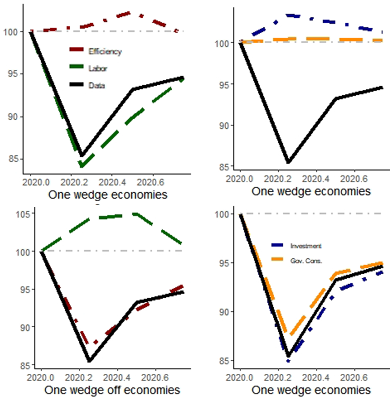
Figure 10. Simulated output trajectory during the COVID crisis. Notes: The red curves are for the model with (without) the efficiency wedge in one-wedge (off) economies; analogously, the green curves are related to the labor wedge, the blue curves to the investment wedge, and the orange curves to the government consumption wedge. The black line is the observed data. 1994Q4 = 100.

Figure 11. The dynamics of output during the COVID crisis: data vs simulations. Notes: In both graphs, the solid line stands for HP-filtered data of output and the dashed line refers to the simulation of the log-linearized version of the detailed economy with the exogenous shocks on the real exchange rate. On the top panel, the simulation is for the 1994Q1–1998Q3 period. On the bottom panel, the simulation is for the 2007Q4–2015Q1 period.


