Coupled Richtmyer–Meshkov and Kelvin–Helmholtz instability on a shock-accelerated inclined single-mode interface

Abstract

The coupling of Richtmyer–Meshkov instability (RMI) and Kelvin–Helmholtz instability (KHI), referred to as RM-KHI, on a shock-accelerated inclined single-mode air–SF$_6$ interface is studied through shock-tube experiments, focusing on the evolution of the perturbation distributed along the inclined interface. To clearly capture the linear (overall linear to nonlinear) evolution of RM-KHI, a series of experiments with a weak (relatively strong) incident shock is conducted. For each series of experiments, various $\theta _{i}$ (angle between incident shock and equilibrium position of the initial interface) are considered. The nonlinear flow features manifest earlier and develop faster when $\theta _{i}$ is larger and/or shock is stronger. In addition, the interface with $\theta _{i}>0^{\circ }$ evolves obliquely along its equilibrium position under the effect of KHI. RMI dominates the early-time amplitude evolution regardless of $\theta _{i}$ and shock intensity, which arises from the discrepancy in the evolution laws between RMI and KHI. KHI promotes the post-early-stage amplitude growth and its contribution is related positively to $\theta _{i}$. An evident exponential-like amplitude evolution behaviour emerges in RM-KHI with a relatively strong shock and large $\theta _{i}$. The linear model proposed by Mikaelian (Phys. Fluids, vol. 6, 1994, pp. 1943–1945) is valid for RM-KHI within the linear period. In contrast, the adaptive vortex model (Sohn et al., Phys. Rev. E, vol. 82, 2010, p. 046711) can effectively predict both the interface morphology and overall amplitude evolutions from the linear to nonlinear regimes.

1. Introduction

The physical process of a shock wave obliquely interacting with an interface separating two fluids with different densities (inclined shock-interface interaction) widely exists in applications such as inertial confinement fusion (ICF) (Nuckolls et al. 1972; Lindl et al. 2014; Betti & Hurricane 2016), scramjet (Billig 1993; Yang, Kubota & Zukoski 1993) and supernova explosion (Maeda et al. 2010; Kuranz et al. 2018). For example, in ICF, the shocks (interfaces) are typically non-centrosymmetric (perturbed) due to the asymmetric drive (limited machining accuracy) (Smalyuk et al. 2005; Edwards et al. 2011; Smalyuk et al. 2020), leading to the occurrence of inclined shock–interface interaction. The waves and interface instability resulting from the inclined shock–interface interaction could significantly influence the implosion of ICF, thus affecting the energy gain and even leading to ignition failure. In scramjet, oblique shock waves reflected between boundaries would interact with the perturbed interface separating fuel from air (Yang et al. 1993; Ren et al. 2019), resulting in the emergence of complex wave configurations and interface instability. The waves would increase the temperature, while the interface instability would enhance the mixing of fuel and air, thereby enhancing the combustion efficiency of the fuel. Therefore, studying the inclined shock–interface interaction is of great significance.

During the inclined shock–interface interaction, shock refraction is a classical physical phenomenon that has been extensively studied for decades. Taub (1947) and Polachek & Seeger (1951) provided the theoretical framework for describing the regular refraction. Subsequently, Jahn (1956) conducted shock-tube experiments on shock refraction with diverse initial conditions, and several irregular shock refraction patterns were observed and discussed. Following up, comprehensive theoretical (Henderson 1966, 2014), experimental (Abd-El-Fattah, Henderson & Lozzi 1976; Abd-El-Fattah & Henderson 1978a,b) and numerical (Henderson, Colella & Puckett 1991; Nourgaliev et al. 2005; Xiang & Wang 2019; de Gouvello et al. 2021) studies on the inclined interaction of a shock wave with a plane or non-planar interface were conducted, and the shock refraction patterns and their transitions have been widely investigated.

The post-shock interface instability resulting from the inclined shock–interface interaction is also a longstanding research focus. Presently, most relevant studies focus on the large-scale perturbation growth, which is regarded as Richtmyer–Meshkov instability (RMI) (Richtmyer 1960; Meshkov 1969) on an inclined interface (inclined-interface RMI). For the inclined-interface RMI, as shown in figure 1(a,b), the equilibrium position of the interface is considered to be perpendicular to the incident-shock-propagation direction, and the initial perturbation is regarded as the entire interface with respect to the equilibrium position, including the perturbations applied to it. Based on a series of numerical studies (McFarland, Greenough & Ranjan 2011, 2013, 2014a), experiments on the inclined-interface RMI at a plane interface, as sketched in figure 1(a), with reshock were conducted using a shock-tube facility at Texas A$\&$M University (McFarland et al. 2014b; Reilly et al. 2015). The membraneless plane interface inclined with respect to the direction of the incident shock propagation was created by tilting the shock tube at an angle relative to the horizontal, while the observation of the pre- and post-reshock flows with high spatiotemporal resolution was realized using the planar laser Mie scattering technique. The dimensionless mixing width was observed to grow linearly in the pre-reshock regime and then level off at the onset of reshock, after which it varies linearly again (McFarland et al. 2014b). In addition, it was found that a more developed pre-reshock interface generally results in a more mixed post-reshock interface (Reilly et al. 2015). Afterwards, by imposing shear and buoyancy on the inclined plane interface to create multi-mode perturbation, experiments on the inclined-interface RMI at a multi-mode interface, as shown in figure 1(b), were performed (Mohaghar et al. 2017, 2019). The evolving density and velocity fields were successfully measured using planar laser-induced fluorescence (PLIF) and particle image velocimetry (PIV) techniques simultaneously. Based on this, the dependencies of the turbulent mixing transition on the initial perturbation (Mohaghar et al. 2017) and incident shock intensity (Mohaghar et al. 2019) were explored.

Figure 1. Sketches of various shock-driven hydrodynamic instabilities. (a) RMI induced by a shock wave interacting obliquely with a plane interface; (b) RMI resulting from the oblique interaction of a shock wave with a multi-mode interface; (c) RMI triggered by a shock wave interacting with a ‘V’-shaped interface; (d) RM-KHI resulting from the inclined interaction between a shock wave and a perturbed interface; (e) RM-KHI resulting from the vertical interaction between a shock wave and a perturbed interface. Red and blue solid lines represent waves and interface, respectively; blue dashed lines denote the interface equilibrium position regarded in relevant research; IS, incident shock; II, initial interface; TS, transmitted shock; RW, reflected wave; SI, shocked interface; $a_0$ and $a$, perturbation amplitudes of II and SI, respectively.

In addition, RMI that occurs when a planar shock interacts with a ‘V’-shaped interface (as shown in figure 1c), which is highly similar to the inclined-interface RMI at a plane interface, has also been studied widely. The dependencies of amplitude evolution on the shock intensity and initial amplitude are the focus of relevant research, and previous works (Sadot et al. 2003; Luo et al. 2016; Guo et al. 2019) indicated that the high-amplitude effect is more significant than the high-Mach-number effect in inhibiting the amplitude growth. In addition, Liang et al. (2019) found that for a shock-accelerated ‘V’-shaped interface, perturbation modes other than the fundamental one also affect the linear growth rate, leading to the failure of the impulsive model (Richtmyer 1960).

The aforementioned investigations have provided valuable insights into the inclined shock–interface interaction from the perspectives of shock refraction and inclined-interface RMI. In addition, the post-shock evolution of the small-scale perturbations distributed along the inclined interface is also interesting. Mikaelian (1994) pointed out that when a shock wave obliquely interacts with a perturbed interface, as depicted in figure 1(d), the normal component of the shock triggers RMI, while its parallel component induces Kelvin–Helmholtz instability (KHI) (Helmholtz 1868; Thompson 1871). The evolution of the small-scale perturbation distributed along the inclined interface, induced by the coupling of RMI and KHI, is referred to as RM-KHI in this work. To avoid confusion, there are several issues that need further clarification. First, the inclined-interface RMI occurs whether the interface is planar or disturbed, whereas RM-KHI can only occur when the interface is perturbed. Second, studies on the inclined-interface RMI consider the inclined interface itself as a component of the initial perturbation, and mainly focus on the large-scale perturbation evolution. In contrast, research on RM-KHI only treats the disturbances distributed along the inclined interface as the initial perturbation, and focuses on the small-scale perturbation evolution. In other words, inclined-interface RMI and RM-KHI could exist simultaneously in the physical process of the inclined shock–interface interaction, but relevant research has different descriptions of physics and different specific objects of concern. Third, when a shock wave propagates vertically along a perturbed interface, RM-KHI, instead of pure shock-driven KHI (Hurricane 2008; Harding et al. 2009; Hurricane et al. 2012; Zhou et al. 2019), still occurs since the transmitted shock induces a velocity normal to the interface as depicted in figure 1(e). Actually, RMI must occur with a shock-driven KHI, though it may be weak when the angle between the shock wave and the equilibrium position of the initial interface ($\theta _{i}$) approaches 90$^{\circ }$. Investigating RM-KHI holds great practical significance due to its widespread presence in ICF and scramjet. It is also significant and interesting to study the perturbation evolution driven by RM-KHI, since the KHI-induced perturbation amplitude growth has a remarkably different law from the RMI-induced one (Richtmyer 1960; Kelly 1965; Harding et al. 2009).

Theoretically, referring to the concept of Richtmyer (1960), Mikaelian (1994) treated the shock as an instantaneous acceleration and developed a linear amplitude evolution model for RM-KHI (the M-L model). Banerjee et al. (2012) studied the bubble (lighter fluids penetrating heavier ones) evolution of RM-KHI in viscous flow using the model of Layzer (1955), and found that the amplitude growth rate of the bubble approaches a finite asymptotic value in the late stages. Experimentally, Rasmus et al. (2018) investigated RM-KHI under High-Energy-Density (HED) conditions on the Omega laser system by obliquely accelerating a sinusoidal C$_{22}$H$_{14}$O$_4$N$_2$–CH foam interface using a laser-driven shock. Based on the X-ray radiographs, it was observed that the perturbation amplitude successively undergoes linear and nonlinear evolution periods. Subsequently, Rasmus et al. (2019) found that neither the discrete vortex model (D-V model) (Hurricane 2008) nor a modified vortex model (M-V model), which additionally considers the vorticity distribution along the interface relative to the D-V model, could accurately predict the amplitude growth observed in HED experiments (Rasmus et al. 2018). The failure of these two models, as pointed out by Pellone et al. (2021), may be largely due to the ignoring of the self-induced evolution and transport of vorticity. Recently, Pellone et al. (2021) theoretically studied RM-KHI under HED conditions using the adaptive vortex model (A-V model) (Sohn, Yoon & Hwang 2010) which overcomes the major shortcomings of the D-V and M-V models. By applying a scaling approach proposed based on the M-L model, Pellone et al. (2021) found that RMI dominates the early-time amplitude growth under various $\theta _{i}$ conditions, and the dynamics dominated by KHI occur earlier and are more pronounced in RM-KHI with larger $\theta _{i}$. Additionally, the A-V model was shown to be capable of predicting the interface morphology and amplitude evolution observed in the HED experiment (Rasmus et al. 2018) when the deceleration and decompression caused by laser turn-off were considered.

Previous studies have shed some light on the evolution law of RM-KHI. In the laser-driven experiment, the materials forming the initial interface are in the solid state and, accordingly, the perturbation on the initial interface can be accurately controlled. However, the perturbation evolution in laser-driven experiments is not solely influenced by hydrodynamic instabilities. For instance, experiments conducted on the Omega laser system generally involve additional physical processes such as the preheat of pre-shocked material (Glendinning et al. 2003), phase transition of solid materials (Malamud et al. 2013) and plasma diffusion (Haines et al. 2014). In addition, the deceleration and decompression caused by laser turn-off also strongly affect the perturbation growth (Rasmus et al. 2018; Pellone et al. 2021). Consequently, isolating the contribution of RM-KHI to the perturbation growth in the laser-driven experiment is challenging. In contrast to the laser-driven experiment, the shock-tube experiment can provide a relatively ‘simple’ physical environment and has therefore become one of the major ways to study shock-driven hydrodynamic instabilities over the last decades (Zhou 2017a,b). Until now, a fine shock-tube experimental study on RM-KHI, focusing on the small-scale perturbation development, is still desirable. The behaviour of RM-KHI under various $\theta _{i}$ conditions and the applicability of existing theoretical models for describing its evolution remain unclear, which motivates the current study.

In this work, some significant parameters directly related to the perturbation growth of RM-KHI are first clarified. Subsequently, RM-KHI is studied through shock-tube experiments using well-defined inclined single-mode gaseous interfaces formed by the soap-film technique (Luo et al. 2016; Liang et al. 2019). Since RM-KHI enters the nonlinear phase rapidly, to sufficiently capture the linear evolution of RM-KHI and verify the linear model, a series of experiments with a weak incident shock is conducted. In addition, a series of experiments with a relatively strong incident shock is performed to clearly obtain the overall evolution law of RM-KHI from the linear to nonlinear stages under diverse $\theta _{i}$ conditions. Finally, the interface morphology and amplitude evolution under various initial conditions are discussed and analysed, and existing models are examined.

2. Clarification of significant parameters

The interaction of a planar incident shock (IS) with an inclined small-amplitude single-mode light-heavy initial interface (II), as depicted in figure 2(a), is considered. Regular refraction is assumed to occur during the IS–II interaction and, accordingly, there are five flow regions (regions 1–5) in the vicinity of the IS–II interaction point. Note that the shock compression alters the perturbation wavelength ($\lambda$), wavenumber ($k=2{\rm \pi} /\lambda$) and amplitude ($a$), and their pre- and post-shock values will be denoted by subscripts ‘0’ and ‘1’, respectively. Four significant parameters directly related to the perturbation growth, including $\lambda _1$, $a_1$, velocity jump that triggers RMI ($\Delta V_{RM}$) and velocity difference that induces KHI ($\Delta V_{KH}$), will be clarified for better understanding RM-KHI.

Figure 2. (a) Interaction of a planar shock with an inclined small-amplitude single-mode light–heavy interface; (b,c) schematics of the determination methods for (b) $\lambda _1$ and (c) $a_1$. Solid and dashed lines represent discontinuities and corresponding equilibrium positions, respectively; line E-IS, extension line of IS; lines FG and HI, auxiliary lines; RS, reflected shock; $a_1$, post-shock perturbation amplitude; $\lambda _0$ and $\lambda _1$, pre- and post-shock perturbation wavelengths, respectively; $\theta _{i}$, angle between IS and the equilibrium position of II; $\theta _{s}$ ($\theta _{t}$), angle between line E-IS and the equilibrium position of SI (TS); $\theta _{ti}$ ($\theta _{ts}$), angle between lines EG (EI) and E-IS; $u$, flow velocity; superscripts 4 and 5 represent the flow regions, and subscripts ‘sn’ and ‘st’ represent the normal and tangential directions to the equilibrium position of SI, respectively.

(1) $\lambda _1$. The shock-compression process of the fluid in region 2 will be analysed to determine $\lambda _1$. Because $k_0a_0$ is small, the compression of $a$ is a ‘microscopic’ process compared with the compression of $\lambda$. Hence, the perturbed shocks and interfaces can be approximated as their equilibrium positions when solving $\lambda _1$. As shown in figure 2(b), when IS moves a distance of $\lambda _0$ along II from points A to B, the pre-shock fluid enclosed by right triangle BAC is compressed by the transmitted shock (TS) into the post-shock fluid enclosed by right triangle BDC. Consequently, we have

(2.1)\begin{equation} \frac{\lambda_1}{\lambda_0}=\frac{\cos (\theta_{i}-\theta_{t})}{\cos(\theta_{s}-\theta_{t})}, \end{equation}

where $\theta _{t}$ ($\theta _{s}$) represents the angle between the equilibrium position of TS (shocked interface SI) and the extension line of IS, which can be determined via shock-polar analysis. Here, $\theta _{t}$ and $\theta _{s}$ are related to $\theta _{i}$ and the shock Mach number ($M$). Accordingly, $\lambda _1$ is correlated with $\lambda _0$, $\theta _{i}$ and $M$.

(2) $a_1$. A section of II with a quarter wavelength, which is approximated as a straight line EG as shown in figure 2(c), is considered to explore the determination method of $a_1$ in RM-KHI. Points E and G are located at the equilibrium position and trough of II, respectively, and point F is the projection of point G onto the equilibrium position. The angle between line EG and the extension line of IS, referred to as $\theta _{ti}$, equals to $\theta _{i}-\arctan (4a_0/\lambda _0)$. SI is approximated as a straight line EI, in which point I corresponds to the trough of SI and point H is the projection of point I onto the equilibrium position. According to the geometric relation, $a_1$ can be determined as

(2.2)\begin{equation} a_1=\frac{\lambda_1}{4}\tan(\theta_{s}-\theta_{ts}), \end{equation}

where $\theta _{ts}$ is the angle between line EI and the extension line of IS, which can be obtained by shock-polar analysis if $\theta _{ti}$ is provided. Here, $\theta _{ts}$ is correlated with $a_0$, $\lambda _0$, $\theta _{i}$ and $M$ and, accordingly, $a_1$ is also related to these parameters.

(3) $\Delta V_{RM}$. Previous studies (Mikaelian 1994; Pellone et al. 2021) stated that RMI in RM-KHI is induced by the shock acceleration perpendicular to the interface. However, it remains unclear whether the interface refers to II or SI. As shown in figure 2(a), the components of the mean velocities of the fluids in regions 4 and 5 ($u^4$ and $u^5$) in the direction normal to SI ($u^4_{sn}$ and $u^5_{sn}$) must be equal due to the interface velocity boundary condition. In contrast, the components of $u^4$ and $u^5$ in the direction tangential to SI ($u^4_{st}$ and $u^5_{st}$) are different owing to the different acoustic impedances of the fluids in regions 1 and 2. Accordingly, the components of $u^4$ and $u^5$ in the direction normal to II ($u^4_{in}$ and $u^5_{in}$) cannot be equal. Since $\Delta V_{RM}$ should be equal for fluids on both sides of the interface, $\Delta V_{RM}$ in RM-KHI should be $u^4_{sn}$ or $u^5_{sn}$ rather than $u^4_{in}$ or $u^5_{in}$.

(4) $\Delta V_{KH}$. KHI occurs when there is a difference in the tangential velocities of the fluids on either side of the interface. For RMI with $\theta _{i}=0^{\circ }$, a shear velocity across the interface always exists as long as there is a perturbation creating a misalignment. From another perspective, KHI is an ‘inherent’ part of RMI, which would result in the generation of the roll-up structure at the nonlinear stage. However, $\Delta V_{KH}$ for RM-KHI refers specifically to the mean velocity difference between fluids on both sides of the interface along the direction of the interface equilibrium position: the difference between $u^4_{st}$ and $u^5_{st}$, i.e. $u^4_{st}$-$u^5_{st}$.

The variations of $\lambda _0$/$\lambda _1$, $a_0$/$a_1$, $\Delta V_{RM}$ and $\Delta V_{KH}$ with $\theta _{i}$ are calculated via shock-polar analysis, considering an air–SF$_6$ interface accelerated by shock waves with different $M$ (1.05, 1.20 and 2.00). The initial pressure and temperature of the pre-shock gases on both sides of II are set as 101.3 kPa and 298.15 K, respectively. As shown in figure 3(a), $\lambda _0$/$\lambda _1$ is weakly positively related to both $M$ and $\theta _{i}$. Nevertheless, when $M$ is 2.0 and $\theta _{i}$ is large, the compression of $\lambda$ by IS is non-negligible. Here, $a_0$/$a_1$ is strongly positively related to $M$, and weakly negatively correlated with $\theta _{i}$ when $M$ is 1.05 or 1.20. When $M$ is 2.0, the correlation of $a_0$/$a_1$ with $\theta _{i}$ is significant. Overall, with the increase of $M$ and $\theta _{i}$, $a_1$ in RM-KHI increasingly differs from that calculated using the method adopted in RMI and $\lambda _1$ also gradually deviates from $\lambda _0$. As illustrated in figure 3(b), $\Delta V_{RM}$ and $\Delta V_{KH}$ are also strongly positively related to $M$, and the former (latter) is weakly negatively (strongly positively) correlated to $\theta _{i}$. Consequently, it can be inferred that RM-KHI evolves faster when $M$ is higher, and the contribution of RMI (KHI) to the amplitude growth of RM-KHI is similar (significantly different) under various $\theta _{i}$ conditions.

Figure 3. Variations of (a) $\lambda _0$/$\lambda _1$ and $a_0$/$a_1$, (b) $\Delta V_{RM}$ and $\Delta V_{KH}$ with $\theta _{i}$.

3. Experimental methods

To realize the inclined interaction between shock wave and perturbed interface in shock-tube experiments, the soap-film technique, which has been extensively verified in previous works (Liu et al. 2018; Li et al. 2023), is employed to create the inclined single-mode air–SF$_6$ interface. As illustrated in figure 4, the transparent interface formation devices (devices A and B) with an inner cross-sectional area of $140\,{\rm mm} \times 6\,{\rm mm}$ are manufactured by combining two acrylic plates with pedestals. The adjacent boundaries of the two devices are machined into the profile of the initial interface perturbation, and two constraint strips, with the same shape as the device boundaries, are affixed to the pre-carved grooves on device B to constrain the soap film. According to our previous work (Wang et al. 2022), when the height ratio of the constraint strips protruding into the flow field to the entire flow field ($\,f$) is 10 %, they would not significantly affect the main part of the shocked interface and the perturbation evolution on it. In the present work, to minimize the potential influence of the constraint strips on interface evolution, $f$ is controlled to be 3 %. To generate the soap film, the constraint strips are first wetted by the soap solution (78 % pure water, 2 % sodium oleate and 20 % glycerin by mass), and then a rectangular frame with the soap solution attached is pulled carefully along the constraint strips. Since $\theta _{i}$ is an acute angle, the soap film near the upper pedestal may deviate from its intended position due to the surface tension effect (Wang, Si & Luo 2013). To address this issue, super-hydrophobic-oleophobic surfaces (Li et al. 2023) are created on the inner edges of two acrylic plates adjacent to the upper pedestal, thus effectively constraining the soap film. For creating an air–SF$_6$ interface, air in device B needs to be replaced with SF$_6$ using the following procedure. First, a thin membrane is used to seal the downstream side of device B, and two pipes are inserted through the membrane into device B. Then, SF$_6$ is charged slowly into device B through the inlet pipe and air is released through the outlet pipe. An oxygen concentration detector is placed at the outlet pipe to monitor the oxygen concentration in device B. Once the volume fraction of oxygen drops below 0.5 %, the pipes are removed, and then the holes on the membrane are sealed. Subsequently, devices A and B are carefully connected and an inclined single-mode air–SF$_6$ interface is formed.

Figure 4. Schematic for the formation of inclined single-mode air–SF$_6$ interface. SHOS, super-hydrophobic-oleophobic surfaces.

A horizontal shock tube, which has been extensively used in prior investigations (Liu et al. 2018; Liang et al. 2019), is applied to generate the planar incident shock wave. Previous studies (Rangel & Sirignano 1988, 1991) showed that the roll-up structure, which is a sign that the interface instability has entered the strongly nonlinear stage, would rapidly emerge in KHI, indicating that the linear evolution of RM-KHI is likely to last only a short period. Therefore, to capture more clearly the linear evolution of RM-KHI and to examine the M-L model, a series of experiments in which a weak IS ($M=1.05\pm 0.01$) is adopted to lower the interface evolution rate is first conducted. Note that to produce such a weak IS, the employed polyester membrane for separating air in the driver and driven sections of the shock tube is very thin (with a thickness of $3.8\,\mathrm {\mu }$m). Then, to obtain the overall evolution law of RM-KHI from the linear to nonlinear stages and to examine the applicability of the A-V model for RM-KHI, a series of experiments with a relatively strong IS ($M=1.20\pm 0.01$) is performed, in which the membrane is of a thickness of $12.5\,\mathrm {\mu }$m. Note that shock waves with $M\approx 1.20$ are described as relatively strong ones in this work to distinguish them from the weaker shock waves with $M\approx 1.05$. Actually, in many applications involving shock-driven interface instability and related scientific research (Zhou 2017a,b; Zhou et al. 2019; Zhou 2021), these are all very weak shock waves. For each series of experiments, four different $\theta _{i}$ of $0^{\circ }$, $10^{\circ }$, $30^{\circ }$ and 50$^{\circ }$ are considered, in which the experiment with $\theta _{i}=0^{\circ }$ serves as the reference case to demonstrate the effect of KHI on interface evolution. Here, $a_0$ and $\lambda _0$ are fixed as 0.27 and 20.00 mm, respectively. Accordingly, II (with $k_0a_0\approx 0.085$) satisfies the small-amplitude criterion ($ka\ll 1$). Note that the experiment with a weak (relatively strong) IS will be referred to as ‘case W-$\theta _{i}$’ (‘case S-$\theta _{i}$’) for clarity.

The evolution of the flow field is captured using a high-speed schlieren system. The schlieren optical arrangement adopted is identical to the one illustrated in the previous work (Chen et al. 2023). In experiments with a weak IS, the high-speed video camera (FASTCAM SA5, Photron Limited) operates at a frame rate of 42 000 frames per second, with the spatial resolution of the schlieren images of approximately 0.21 mm pixel$^{-1}$. In experiments with a relatively strong IS, the camera operates at a frame rate of 50 000 frames per second, with the spatial resolution of the schlieren images of approximately 0.39 mm pixel$^{-1}$. The exposure time of the camera is fixed as $1\,\mathrm {\mu }$s. The temperature and pressure of the pre-shock gases in the test section (air and SF$_6$) are identical to their ambient counterparts: $101.3\pm 0.1$ kPa and $298.4\pm 0.5$ K, respectively.

Table 1 presents some significant parameters of eight experimental cases with various initial conditions, in which superscripts ‘$e$’ and ‘$t$’ denote the experimental and theoretical results, respectively, and similarly hereinafter. Experimentally, the velocity of IS ($v_{IS}$), $\theta _{s}$ and $\theta _{t}$ are first measured from schlieren photographs. Then, the velocity of TS ($v_{TS}$) and $\Delta V_{RM}$ can be calculated using geometric relationships. Theoretically, assuming that the fluid in region 1 is pure air, the composition of the fluid in region 2 and the post-shock Atwood number ($A_1=(\rho ^5-\rho ^4)/(\rho ^5+\rho ^4)$, with $\rho ^4$ and $\rho ^5$ being the densities of the fluids in regions 4 and 5, respectively) are determined by matching $v_{TS}^e$ and $v_{TS}^t$. Other significant parameters are also determined through shock-polar analysis. The relative error between $\Delta V_{RM}^e$ and $\Delta V_{RM}^t$ is less than 4.3 %, indicating that the constraint strips have limited effect on the post-shock flow. Subsequently, considering the good agreement between $\Delta V_{RM}^e$ and $\Delta V_{RM}^t$, the hard-to-obtain $\Delta V_{KH}^e$ is deduced to be approximately equal to $\Delta V_{KH}^t$ determined through shock-polar analysis. The constraint strips embedded on the interface formation device cause II to appear thick (see figures 5 and 6). In experiments with a weak IS, SI moves slowly and takes a while to separate from the dark area caused by constraint strips (112, 115, 67 and $69\,\mathrm {\mu }$s for cases W-0, W-10, W-30 and W-50, respectively), causing the difficulty in accurately extracting $\lambda _1^e$ and $a_1^e$. Therefore, $\lambda _1^e$ and $a_1^e$ have not been provided to compare with the theoretical counterparts. For experiments with a relatively strong IS, $\lambda _1^e$ and $a_1^e$ are provided since the relatively fast movement of SI enables relatively accurate extraction of them. The good agreement between $\lambda _1^e$ and $\lambda _1^t$ ($a_1^e$ and $a_1^t$) verifies the theoretical determination method of $\lambda _1$ ($a_1$).

Table 1. Some significant parameters for eight experimental cases with various initial conditions. Superscripts ‘$e$’ and ‘$t$’ denote experimental and theoretical results, respectively. $v_{IS}$ and $v_{TS}$, velocities of IS and TS, respectively; $A_1$, post-shock Atwood number; $\Delta V_{RM}$, velocity jump that triggers RMI; $\Delta V_{KH}$, velocity difference that induces KHI; $\lambda _1$ and $a_1$, post-shock wavelength and amplitude, respectively; $\gamma _{KHI}$ ($\gamma _{RMI}$), strength (mean strength) of the vortex sheet driving KHI (RMI). Units of length and velocity (or vortex-sheet strength) are mm and m s$^{-1}$, respectively.

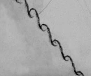
Figure 5. Schlieren photographs of four experimental cases with a weak IS: (a) W-0; (b) W-10; (c) W-30; and (d) W-50. SPP, specific periodic perturbation; RTS, reflected shock wave of TS from the wall. Numbers represent time in $\mathrm {\mu }$s.

Figure 6. Schlieren photographs of experimental cases with a relatively strong IS: (a) S-0; (b) S-10; (c) S-30; and (d) S-50.

4. Results and discussion

4.1. Interface morphologies and flow features

Figures 5 and 6 show the schlieren images of experimental cases with a weak IS and a relatively strong IS, respectively. For clarity, the constraint strips are removed from the images through image processing once the IS–II interaction ends. In experiments with $\theta _{i}>0^{\circ }$, the perturbations on SI exhibit different evolution states, depending on the moment at which IS interacts with them. In this study, we will focus on the evolution of the specific periodic perturbation (SPP) depicted in figures 5 and 6, and the temporal origin is defined as the moment when the whole SPP is affected by IS.

For experiments with a weak IS, cases W-0 and W-30 are taken as examples to illustrate the evolution features. In case W-0, the interaction of IS with II generates TS and RS ($208\,\mathrm {\mu }$s). RS can barely be observed due to its weak intensity. Subsequently, SI evolves slowly and maintains a quasi-single-mode shape throughout the experiment (208–874 $\mathrm {\mu }$s). Note that since the interface evolution is driven solely by RMI, the interface remains symmetrical with respect to its crest or trough, in which the crest (trough) represents the upstream (downstream) point on the interface furthest from the equilibrium position. In case W-30, regular refraction occurs when IS meets II, resulting in the generation of inclined TS and RS (162 $\mathrm {\mu }$s), in which RS cannot be identified due to its weak intensity. In the early stages, SI grows nearly symmetrically with respect to its crest or trough and maintains a quasi-single-mode shape (233–400 $\mathrm {\mu }$s). Subsequently, SI gradually tilts with respect to its crest or trough under the effect of KHI (733 $\mathrm {\mu }$s). Meanwhile, the nonlinear features of interface evolution, such as bubble and spike (heavier fluids penetrating lighter ones), emerge on SI. Overall, the nonlinear flow features in cases with larger $\theta _{i}$ manifest earlier and develop faster compared with those in cases with smaller $\theta _{i}$, which should be attributed to the larger contribution of KHI to perturbation evolution.

For experiments with a relatively strong IS, the IS–II interaction and interface evolution trend are similar to those in experiments with a weak IS, and the nonlinear flow features also manifest earlier and develop faster when $\theta _{i}$ is larger. However, the flattening of the bubble and the thinning of the spike are considerably faster relative to those in experiments with a weak IS. Specifically, in cases S-30 and S-50, an inclined developed roll-up structure, which is a typical nonlinear flow feature in KHI, emerges in the late stages. In cases W-50 and S-50, a reflected shock generated when the inclined TS encounters the upper boundary (RTS) and its interaction with SPP can be observed. The evolution of RTS is a complex shock-dynamic problem, and quantifying its effect on the interface evolution is challenging. Therefore, for cases W-50 and S-50, the effective experimental time ends when SPP is affected by RTS.

4.2. Amplitude evolution

Temporal variations of perturbation amplitude $a$ in dimensionless form for experiments with a weak IS and a relatively strong IS are shown in figure 7(a,b), respectively, in which $t$ is normalized as $\tau$=$k_1^t \dot {a}^{RM} t$, with $\dot {a}^{RM}$ ($=k_1^t A_1 a_1^t \Delta V_{RM}^t$) being the amplitude growth rate predicted by the linear model for RMI, and $a$ is normalized as $\alpha =k_1^t (a-a_1^t)$. Additionally, the predictions of the linear models for RMI and KHI (LP-RMI and LP-KHI) are provided as references. The linear model for RMI is the well-known impulsive model (Richtmyer 1960) which can be written as

(4.1)\begin{equation} a^{RM}(t) = a_1^t + k_1^t A_1 a_1^t \Delta V_{RM}^t t. \end{equation}

The linear model of shock-induced KHI (Kelly 1965; Wang et al. 2021) can be expressed as

(4.2)\begin{equation} a^{KH}(t) = a_1^t \cosh(\varepsilon t), \end{equation}

where $\varepsilon =k_1^t \Delta V_{KH}^t \sqrt {1-{A_1}^2}/2$. Note that due to the scaling approach employed, LP-RMI for different cases are the same in dimensionless form. It can be found that the scaling approach, which has been proven to apply to RMI on a small-amplitude single-mode interface (Liu et al. 2018), can also collapse the amplitude evolutions of RM-KHI under diverse $\theta _{i}$ and $M$ conditions in the early stages. In addition, the early-time results of all experimental cases agree reasonably with LP-RMI, indicating that RMI dominates the early-time amplitude evolution of RM-KHI regardless of $\theta _{i}$ and $M$. This phenomenon arises from the disparity in the evolution laws between RMI and KHI: the amplitude growth rate ($\dot {a}$) induced by RMI increases rapidly from zero to an asymptotic value (Richtmyer 1960; Velikovich, Herrmann & Abarzhi 2014), whereas KHI-induced $\dot {a}$ follows an exponential law rising slowly from zero during the early stages (Kelly 1965; Drazin & Reid 1981).

Figure 7. (a,b) Experimental amplitude evolutions (Exp) and predictions of linear models for RMI and KHI (LP-RMI and LP-KHI); (c,d) initial vortex-sheet strength distributions (IVSDs) for different cases.

To better understand the post-early-stage amplitude evolution, the initial vortex-sheet strength distribution (IVSD) is calculated by predicting the local deposited vortex-sheet strength ($\gamma$) using the formula proposed by Samtaney & Zabusky (1994) via shock-polar analysis:

(4.3)\begin{equation} \gamma={\frac{2c}{Q+1}}(1-\sigma^{-({1}/{2})})(1+ M^{{-}1}+2 M^{{-}2})(M-1)\sin\theta_{d}, \end{equation}

where $c$ is the sound speed of the fluid in region 1; $\sigma$ and $Q$ are the density ratio and average specific heat ratio of the fluids in regions 1 and 2, respectively; $\theta _{d}$ is the local angle between IS and II. IVSDs for experiments with a weak IS and a relatively strong IS are shown in figures 7(c,d), respectively, in which $\Delta \gamma _{max}$ and $\Delta \gamma _{min}$ represent the deviations of the maximum and minimum values of $\gamma$ from its average value ($\gamma _{KHI}$), respectively, and $x$ denotes the coordinate along the direction tangential to the equilibrium position of SI. Here, $\gamma _{KHI}$ $(\gamma _{RMI}=(\Delta \gamma _{max}+\Delta \gamma _{min})/2)$ represents the strength (mean strength) of the vortex sheet driving KHI (RMI), and the magnitudes for different cases are listed in table 1. Interestingly, for a given $\theta _{i}$, $\gamma _{KHI}$/$\gamma _{RMI}$ in the two series of experiments are almost identical, indicating that $\gamma _{KHI}$/$\gamma _{RMI}$ is mainly determined by $\theta _{i}$ and is insensitive to $M$. The amplitude evolution in cases W-0 and S-0 exhibits a quasi-linear behaviour, which aligns with the interface morphologies shown in figures 5(a) and 6(a). For case W-10, the amplitude evolution is almost identical to that in case W-0. For case S-10, the amplitude evolution exhibits a comparable quasi-linear behaviour to that in case S-0, and their discrepancy is negligible until the late stages. Moreover, LP-KHI is limited within the time period considered. These results indicate that the effect of KHI on amplitude evolution is weak when $\gamma _{KHI}$ is comparable to $\gamma _{RMI}$. For cases W-30 and W-50, the amplitude growth deviates gradually from that in case W-0, and the deviation occurs earlier when $\theta _{i}$ is larger. For cases S-30 and S-50, the amplitude growth deviates significantly from that in case S-0 and exhibits an evident exponential-like behaviour shortly after the initial stages. In addition, LP-KHI becomes significant rapidly. These observations illustrate that when $\gamma _{KHI}$ is significantly higher than $\gamma _{RMI}$, KHI would considerably promote the amplitude growth and even alter the amplitude evolution law. In the late stages of cases S-30 and S-50, $\dot {a}$ reduces due to nonlinearity, as evidenced by the significant nonlinear features of the interface shown in figure 6(c,d).

In addition to the small-scale perturbation evolution driven by RM-KHI, the large-scale perturbation growth of the inclined-interface RMI is also of significance for understanding the interface evolution. In the present experiments, due to the spatial constraints of the observation windows, the upper and lower boundaries of the flow field are not included within the observation region, and the large-scale perturbation evolution cannot be obtained. Therefore, the large-scale perturbation growth is discussed via numerical simulations, as presented in Appendix A.

4.3. Model evaluation

4.3.1. Linear model

In the series of experiments with a weak IS, $k_0a_0$ satisfies the small-amplitude criterion and a sufficient amount of experimental data is obtained within a sufficiently small $\tau$. Therefore, these experiments are suitable for validating the linear model of RM-KHI. The linear model proposed by Mikaelian (1994), i.e. the M-L model, can be written as

(4.4)\begin{equation} a^{ML}(t) =a_1^t \left[\cosh(\varepsilon t )+{\frac{k_1^t A_1 \Delta V_{RM}^t}{\varepsilon}}\sinh(\varepsilon t)\right]. \end{equation}

It is worth mentioning again that the M-L model addresses the linear regime and is not expected to be valid when nonlinearity becomes significant. Therefore, to examine the M-L model, it is essential to know when RM-KHI enters the nonlinear evolution phase. It is very challenging to determine when the linear-to-nonlinear transition occurs from the amplitude evolution because RMI and KHI, which have significantly different amplitude evolution patterns, exist simultaneously. Qualitatively, in RMI, when the interface grows asymmetrically with respect to its equilibrium position (as shown in figure 8a), i.e. the amplitude growths of the spike and bubble exhibit a certain difference, the interface evolution is considered to enter the nonlinear regime (Collins & Jacobs 2002; Niederhaus & Jacobs 2003; Liu et al. 2018). In KHI, when the interface becomes asymmetric with respect to its crest or trough (as shown in figure 8b), with bubble flattening and spike thinning, the interface evolution is considered to be within the nonlinear regime (Pullin 1982; Wang et al. 2009). According to previous works on KHI (Rangel & Sirignano 1988, 1991) and RMI (Niederhaus & Jacobs 2003; Vandenboomgaerde et al. 2014), the interface perturbation is smaller in the presence of significant nonlinearity in KHI compared with that in RMI. In other words, in RM-KHI, the nonlinear interface feature caused by KHI is likely to occur earlier than that caused by RMI. Therefore, it is reasonable to determine the linear-to-nonlinear transition of RM-KHI using the qualitative criterion of KHI (i.e. the interface becomes asymmetric with respect to its crest or trough).

Figure 8. Sketches of the qualitative feature of an interface as it enters the nonlinear evolution period: (a) RMI; (b) KHI.

The comparison between the amplitude evolutions obtained from experiments with a weak IS and predicted by the M-L model is illustrated in figure 9(a). For case W-0 in which only RMI exists initially, the M-L model degenerates into the impulsive model. A good agreement between the experimental and theoretical results is reached since the interface evolution is still within the linear stage when $\tau <0.3$ (Niederhaus & Jacobs 2003; Liu et al. 2018). For case W-10, the M-L model predicts the amplitude evolution well throughout the effective experimental time. In contrast, the M-L model overestimates the results of cases W-30 and W-50 in the late stages. For cases W-30 and W-50, the interface contour corresponding to the experimental data point where the M-L model overestimates the experimental amplitude by over 10 % is extracted from the schlieren image and shown in figure 9(b), where $y$ denotes the coordinate along the direction normal to the equilibrium position of SI, and the results for different cases are shifted to different $y$ coordinates for better comparison. The interface morphology corresponding to the last effective experimental data point in case W-10 is also provided for comparison. A parameter $\beta$ ($=2L_{\rm CT}/\lambda _1$) is introduced to characterize the degree of the interface asymmetry with respect to the crest or trough. As shown in figure 9(b), $L_{CT}$ represents the distance between the highest point near the crest and the lowest point in the vicinity of the trough along the interface equilibrium position. Note that if $\beta >0.9$ ($\beta <0.8$), it indicates that the interface is almost symmetrical (evidently asymmetrical) with respect to its crest or trough. Here, $\beta$ of the interface contours corresponding to cases W-10, W-30 and W-50 shown in figure 9(b) are $0.94\pm 0.04$, $0.79\pm 0.06$ and $0.73\pm 0.09$, respectively, indicating that the M-L model is accurate within the linear regime and loses accuracy after the interface evolution enters the nonlinear stage. To the authors’ knowledge, this is the first direct validation of the M-L model.

Figure 9. (a) Comparison between amplitude evolutions obtained from experiments with a weak IS and predicted by the M-L model (ML); (b) experimental interface contour corresponding to the last data point or the data point where the M-L model significantly overestimates the experimental result.

4.3.2. Vortex model

Up to now, RM-KHI still lacks an analytical nonlinear model due to the complexity of its physical process and the inadequacy of physical understanding. In this study, the A-V model (Sohn et al. 2010), which considers the evolution of SI as a pure vortex dynamics process, is examined for its capability in describing the overall linear to nonlinear evolution of RM-KHI via the series of experiments with a relatively strong IS. The A-V model has been applied in theoretical studies on KHI (Sohn et al. 2010) and RM-KHI (Pellone et al. 2021), which, in principle, is capable of forecasting the interface evolution to a strongly nonlinear stage at which the roll-up structure emerges. The steps employed in the present study to apply the A-V model to RM-KHI are outlined as follows. First, IVSD is determined using the method described in § 4.2. Then, the evolution of $\gamma$ is solved using the equation derived by Tryggvason (1988):

(4.5)\begin{equation} {\frac{{\rm d}\gamma}{{\rm d} t}} =2A_1\frac{{\rm d}\boldsymbol{U}}{{\rm d} t}\boldsymbol{\cdot} \boldsymbol{s}+\frac{\phi+A_1}{4}\frac{\partial \gamma^2 }{\partial s}-(1+\phi A_1) \gamma \frac{\partial\boldsymbol{U}}{\partial s}\boldsymbol{\cdot} \boldsymbol{s}, \end{equation}

where $\phi$ is an artificial weighting parameter; $\boldsymbol {s}$ is the unit tangent vector at SI; $\boldsymbol {U}=(\boldsymbol {u}^i-\boldsymbol {u}^j)/2$, with $\boldsymbol {u}^i$ and $\boldsymbol {u}^j$ being the velocity vectors of the fluids in regions 4 and 5 at SI, respectively. Subsequently, the vortex-sheet velocity, as well as the interface morphology, are given by the ‘$\delta$ equations’ (Krasny 1986) as

(4.6)$$\begin{gather} u=\frac{1}{2 \lambda_1^t }{\displaystyle\int_{0}^{\lambda_1^t} \frac{\sinh( k_1^t y-k_1^ty')}{\cosh (k_1^ty-k_1^ty')- \cos (k_1^tx-k_1^tx')+\delta^2}} \gamma' \,{\rm d} s', \end{gather}$$

(4.7)$$\begin{gather}v={-}{\frac{1}{2 \lambda_1^t}}{\displaystyle\int_{0}^{\lambda_1^t} \frac{\sin (k_1^tx-k_1^tx')}{\cosh (k_1^ty-k_1^ty')- \cos (k_1^tx-k_1^tx')+\delta^2}} \gamma' \,{\rm d} s', \end{gather}$$

where $u$ and $v$ are the velocity components in the $x$ and $y$ directions, respectively; $\delta$ is a desingularization parameter. When numerically solving the system of equations to obtain the temporal evolutions of interface morphology and perturbation amplitude, all variables are operated in the dimensionless form (Sohn et al. 2010; Pellone et al. 2021). The coordinates $x$ and $y$ are scaled as $x/\lambda _1^t$ and $y/\lambda _1^t$, respectively, while the time $t$ and $\gamma$ are normalized as $\gamma _{max}t/\lambda _1^t$ and $\gamma /\gamma _{max}$, respectively, in which $\gamma _{max}$ is the maximum value of IVSD calculated by (4.3). The vortex sheet is discretized into 400 Lagrangian points, and the dimensionless time step is set to 0.0002. To address simulation failure caused by significant non-uniformity in the distribution of point vortices, a point vortex insertion method is applied when the arclength between two point vortices exceeds a threshold of 0.0125 (Sohn et al. 2010). Here, $\delta$ and $\phi$ are respectively set as 0.15 and $-A_1^2$ (Kerr 1988; Matsuoka & Nishihara 2006; Sohn et al. 2010) to ensure prediction accuracy and sufficient effective simulation time.

The comparison between the interface contours extracted from experimental schlieren photographs and predicted by the A-V model is shown in figure 10, in which the results corresponding to different moments are shifted to different $y$ coordinates for clear presentation. The A-V model can reasonably predict the overall evolution of the interface morphology for all cases, even the interface has entered the strongly nonlinear evolution period. The discrepancies in the details of the roll-up structure between experimental and theoretical results can be partially attributed to the limited resolution and sensitivity of the high-speed schlieren photography compared with advanced diagnostic methods such as PLIF (Collins & Jacobs 2002; Jacobs & Krivets 2005) and simultaneous PLIF/PIV techniques (Mohaghar et al. 2017, 2019). The comparison between the amplitude evolutions obtained from experiments and predicted by the A-V model is shown in figure 11. The predictions of the M-L model are also provided. For cases with $\theta _{i}>0^{\circ }$, the deviation of the experimental data from the prediction of the M-L model is significant at the late stages, indicating that the interface evolution has entered the nonlinear stage. A good agreement between the experimental data and predictions of the A-V model is reached, indicating that the A-V model is capable of predicting the amplitude evolution from the linear to nonlinear stages. Overall, the A-V model describes the linear to nonlinear evolution of RM-KHI well in both qualitative and quantitative terms, indicating that the vortex dynamics is the dominant physical mechanism of RM-KHI.

Figure 10. Interface contours extracted from experiments with a relatively strong IS (solid lines) and predicted by the A-V model (dashed lines): (a) S-0; (b) S-10; (c) S-30; and (d) S-50.

Figure 11. Comparison between amplitude evolutions obtained from experiments with a relatively strong IS and predicted by the M-L model (ML) and A-V model (AV).

5. Conclusions

The coupling of Richtmyer–Meshkov instability (RMI) and Kelvin–Helmholtz instability (KHI), referred to as RM-KHI in the present work, is finely studied in a shock-tube facility by accelerating an inclined single-mode air–SF$_6$ interface using a planar shock wave. We aim to explore the instability behaviour under different angles $\theta _{i}$ (angle between incident shock wave and equilibrium position of the initial interface), and to evaluate the existing theories. The soap-film and super-hydrophobic-oleophobic surface techniques are employed to create well-defined desirable inclined initial interfaces. Since RM-KHI enters the nonlinear stage rapidly, to clearly capture the linear evolution of RM-KHI, a series of experiments in which a weak incident shock is employed to slow down the interface evolution is conducted. In addition, a series of experiments with a relatively strong incident shock is performed to obtain the overall linear to nonlinear evolution of RM-KHI.

The nonlinear flow features manifest earlier and develop faster when $\theta _{i}$ is larger and/or incident shock is stronger. In addition, the interface in RM-KHI with $\theta _{i}>0^{\circ }$ tilts gradually with respect to its crest or trough under the effect of KHI. Specifically, an inclined developed roll-up structure, which is a typical nonlinear flow feature in KHI, emerges in the late stages of experiments with a relatively strong incident shock and large $\theta _{i}$. RMI dominates the amplitude evolution in the early stages regardless of $\theta _{i}$ and shock intensity, which arises from the discrepancy in the evolution laws between RMI and KHI. KHI promotes the post-early-stage amplitude growth and its contribution is related positively to $\theta _{i}$. An evident exponential-like amplitude evolution behaviour emerges in RM-KHI with a relatively strong incident shock and large $\theta _{i}$. By determining the linear-to-nonlinear transition of RM-KHI from the degree of the interface asymmetry with respect to the crest or trough, the linear model proposed by Mikaelian (1994) (M-L model) is proven to be valid in describing the linear amplitude evolution of RM-KHI. Encouragingly, the adaptive vortex model (A-V model) (Sohn et al. 2010) is capable of forecasting the large-scale interface structures and amplitude evolution from the linear stage to the strongly nonlinear stage, indicating that the vortex dynamics is the dominant physical mechanism of RM-KHI. To the authors’ knowledge, this is the first direct validation of the M-L model and the first application of the A-V model to RM-KHI on a single-mode light–heavy interface accelerated obliquely by a shock wave.

In the following work, more shock-tube experiments will be conducted considering different initial conditions, and the evolution law of a heavy–light perturbed interface accelerated obliquely by a shock wave will be explored. Furthermore, for shock-driven interface instability, the schlieren technique is capable of capturing the evolution of the interface and waves. However, it is still challenging to obtain flow information such as the global velocity and vorticity fields through the schlieren results. Therefore, more advanced measurement techniques, such as the PIV and PLIF techniques, will be applied to experiments on shock-driven interface instability, hoping that our experiments can be more useful to numerical developers.