1 - Invasion Science 1.0

Summary

At the time of writing this book, we have witnessed an extreme case of biological invasion. A virus, through an evolutionary leap, has jumped onto a new host species, Homo sapiens, and has taken advantage of the new host’s ambitions and mobility in the zealous phase of globalisation, causing a worldwide pandemic and economic meltdown. The 2019 coronavirus outbreak (COVID-19) is a showcase of the core of invasion science. A list of questions spring to mind. Why this particular virus, and not others? Why now? How fast can it spread? How is its spread mediated by climatic and other environmental factors? What are its vectors and pathways of transmission? Which regions and populations are most susceptible? How much damage can it cause to public health and economies? What factors cause substantial variation in mortality between human populations in different countries? How can we control it? Can we forecast and prevent future outbreaks of emerging infectious diseases? While the whole world scrambles to make sense of COVID-19 and to combat the biggest crisis for humanity since World War II (WWII), we embark on a journey to address these questions to cover many more taxa and situations – the invasion of any biological organism into novel environments.

This [invasion] velocity is proportional to the square root of the intensity of selective advantage and to the standard deviation of scattering in each generation.

(Fisher 1937)

1.1 Welcome to the Anthropocene

At the time of writing this book, we have witnessed an extreme case of biological invasion. A virus, through an evolutionary leap, has jumped onto a new host species, Homo sapiens, and has taken advantage of the new host’s ambitions and mobility in the zealous phase of globalisation, causing a worldwide pandemic and economic meltdown. The 2019 coronavirus outbreak (COVID-19) is a showcase of the core of invasion science. A list of questions spring to mind. Why this particular virus, and not others? Why now? How fast can it spread? How is its spread mediated by climatic and other environmental factors? What are its vectors and pathways of transmission? Which regions and populations are most susceptible? How much damage can it cause to public health and economies? What factors cause substantial variation in mortality between human populations in different countries? How can we control it? Can we forecast and prevent future outbreaks of emerging infectious diseases? While the whole world scrambles to make sense of COVID-19 and to combat the biggest crisis for humanity since World War II (WWII), we embark on a journey to address these questions to cover many more taxa and situations – the invasion of any biological organism into novel environments.

All species have the means to shift their progeny, either via direct movement or through vector-mediated dispersal. The incentive to move has driven Earth’s biota to cover all possible niches, from the Antarctic to the Arctic, from the Himalayas to the Mariana Trench. Most propagules, however, move slowly and over short distances. On very rare occasions do propagules catch a ride on ocean rafts or hurricanes, or become attached to a seabird. Such propensity and limitation of dispersal are key factors behind the world’s distinct biotic zones. This process of natural dispersal and spread of species was altered by early hominids. Hunter-gatherer societies had deep knowledge of the animals and plants around them and started to cultivate many species to ensure a sustainable supply of food and fibre. When humans began colonising the entire planet, cultivated plants and animals moved with them, the result being a growing list of species able to thrive in human-dominated environments, with the capacity to transform landscapes. Not only did humans intentionally move many species with them to supply their needs, but their movements also resulted in the accidental movement of many species. These include species associated with useful organisms, such as yeasts, viruses and other microorganisms, and many other types of pest and weed that simply ‘hitched a ride’ on diverse means of transport. Human selection has resulted in a rather unique assemblage of species, distinct from those that occur in natural communities and which are filtered by natural selection.

Human-mediated movement of species has accelerated dramatically in the era of globalisation, in terms of quantity, distance and speed. Technological innovations have revolutionised ways in which we transport goods. Stretching from Xi’an to Rome, the Silk Road connected the Eurasian supercontinent as early as the first century BC, carrying goods on the backs of horses and camels. Islamic merchants created the Spice Route in the seventh century, thereby connecting the Mediterranean Sea and the Indian Ocean. Global trade started in earnest in the Age of Discovery, when European explorers connected East and West with the Americas in the fifteenth century. Global trade scaled up after the first Industrial Revolution in the eighteenth and nineteenth centuries when global production chains began compartmentalising (e.g. meat export from South America). The trajectory has been interrupted only by two World Wars and the COVID-19 pandemic. After WWII, globalisation resumed its march with the mainstream transport of cars, ships and planes (global export totalling US$62 billion in 1950), only being slowed temporarily by the Iron Curtain during the Cold War. A milestone of this globalisation was the launch of the World Trade Organisation in 1995, when global exports reached US$5 trillion. Globalisation then soared over the next two decades, with bumps along the way during the 2008 recession and the COVID-19 pandemic, reaching close to US$19 trillion in 2014. Real gross domestic product (GDP) per capita in the United States in 2014 was four times the size it was in 1950. The human population increased from 2.5 billion in 1950 to 7 billion in 2012 (Figure 1.1), and is projected to reach 10 billion in 2050. Not only has our ecological footprint overshot the planet’s carrying capacity, but there are also emerging global crises that are threatening the whole of humanity (e.g. climate change, biodiversity loss and the pandemic).

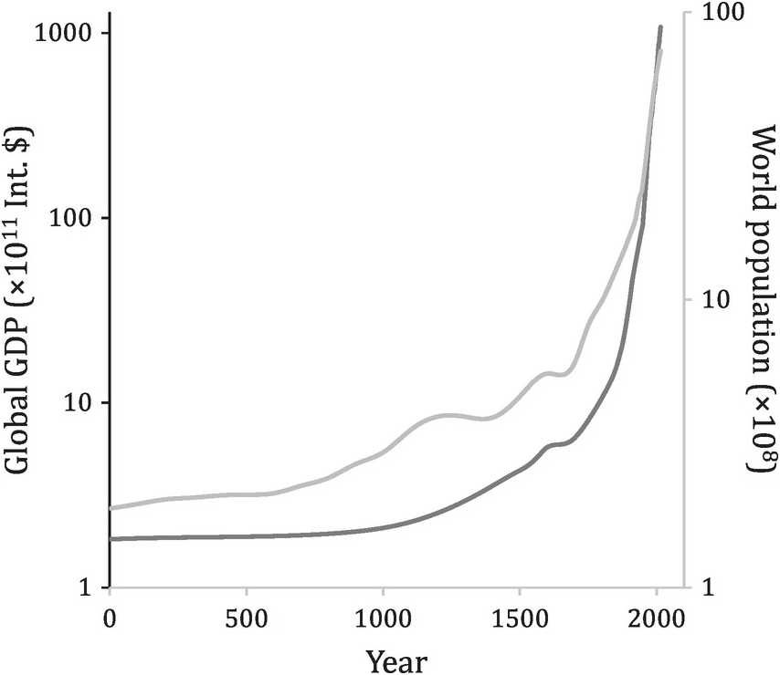
Figure 1.1 Global GDP, in international dollars (2011 price), and world population, in the past two millennia.

Based on data from ourworldindata.org under CC-BY Licence.

With the rising dominance of humans in the biosphere, previously characteristic floras and faunas in regional biotic zones have been mixed and reshuffled, resulting in a major homogenisation of the world’s biota. The accumulation of non-native species across the globe is continuing with no sign of a slowing of the rate of new records of naturalisation and invasion (Seebens et al. 2017). Putting aside biases in taxonomy and sampling effort, the trend in the global rate of new records of established non-native species is overwhelming (Figure 1.2). Geographic and taxonomic variations in the dynamics and rate of non-native establishment reflect the role and history of regional countries in global trade. With the rise of global trade, the rate of establishment of non-native species has increased steadily, as stowaways, contaminants and pets since 1800, and accelerated further after 1950 – with the sole exception of mammals and fishes, which exhibit a hump-shaped curve, perhaps due to the regulations on farming for the game and fur industry. The establishment of non-native plant species has maintained a high rate since 1900 (Figure 1.2), coinciding with acclimatisation and colonisation activities in European diasporas. Technology has enabled us to move species around the world in new ways, quickly and in huge numbers; and changing fashions, fads and desires of human societies are continuously modifying and expanding the catalogue of translocated species – not just for essential goods but also for peculiar luxuries and hobbies. We need new ways of categorising and managing the new assemblages of biota that occur in different environments. Not only do we need to understand how many species are moved around the world by humans, but we also need to understand how these species interact with other species and how the added species and the changes that they bring affect the functioning of ecosystems, and thereby influence our well-being, both positively and negatively.

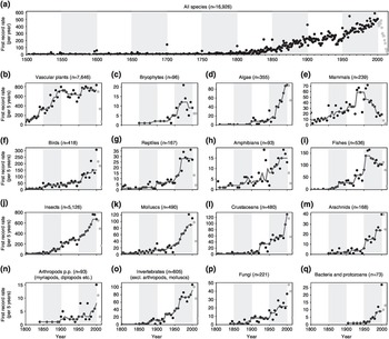
Figure 1.2 Global temporal trends in the rates of first records of the establishment of non-native species. Global temporal trends in first record rates (dots) for all species (a) and taxonomic groups (b–q) with the total number of established non-native species during the respective time periods given in parentheses. Data after 2000 (grey dots) are incomplete because of the delay between sampling and publication, and therefore not included in the analysis. As first record rates were recorded on a regional scale, species may be included multiple times in one plot. (a) First record rates are the number of first records per year during 1500–2014. (b–q) First record rates constitute the number of first records per 5 years during 1800–2014 for various taxonomic groups. The trend is indicated by a running median with a 25-year moving window (red line). For visualisation, 50-year periods are distinguished by white/grey shading.

From Seebens et al. (2017) under CC-BY Licence.

Biological invasions are by no means the only driver of the massive global-scale environmental changes that we are seeing. Invasive species interact in complex ways with other key builders and shapers of novel ecosystems such as agriculture, urbanisation, altered biogeochemical cycles, excessive carbon emission and pollution. For instance, of the documented 291 records of plant species extinction (Le Roux et al. 2019), agriculture, urbanisation, grazing, habitat degradation and destruction, together with biological invasions, are found to be implicated. The exact role of each of these factors is difficult to discern in most cases, but each surely has its own distinct temporal pattern and role to play (Figure 1.3). With these burgeoning factors affecting the planet’s biosphere, we are witnessing pervasive alterations to physical systems, disturbance regimes and biogeochemical cycles, leading to a downward spiral in the integrity and health of ecosystems, accompanied by biodiversity loss and ecosystem transformation. In some cases, biological invasions are directly responsible for the decline of native biota, e.g. native plant species in Mediterranean-type ecosystems have been severely affected by non-native plants, particularly by Australian acacias (Figure 1.4; Gaertner et al. 2009). Recent reviews on the role of biological invasions in reducing the biodiversity of recipient ecosystems overwhelmingly support this view of the detrimental role of invasive species, more so at local than regional levels (Figure 1.5; Chase et al. 2018). These forces of change sometimes reinforce each other at different spatial and temporal scales, often with lags, leading to complex and intertwined challenges to the well-being of humanity and ecosystems (Díaz et al. 2015; Essl et al. 2015a). On this wagon of humanity, many hitchhiker species proliferate, creating harmful impacts on human well-being. The huge number of species that have been transported by us in different quantities and rates, intentionally or not, directly or not, define the subject and context of invasion science (Pyšek et al. 2020a).

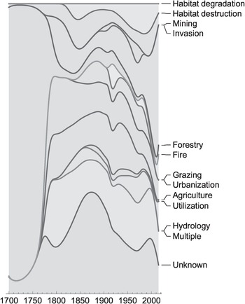
Figure 1.3 Primary drivers of plant extinctions over the last 300 years shown as area graphs to visualise the temporal changes in the relative contribution of the 11 identified primary extinction causes.

Data from Le Roux et al. (2019).

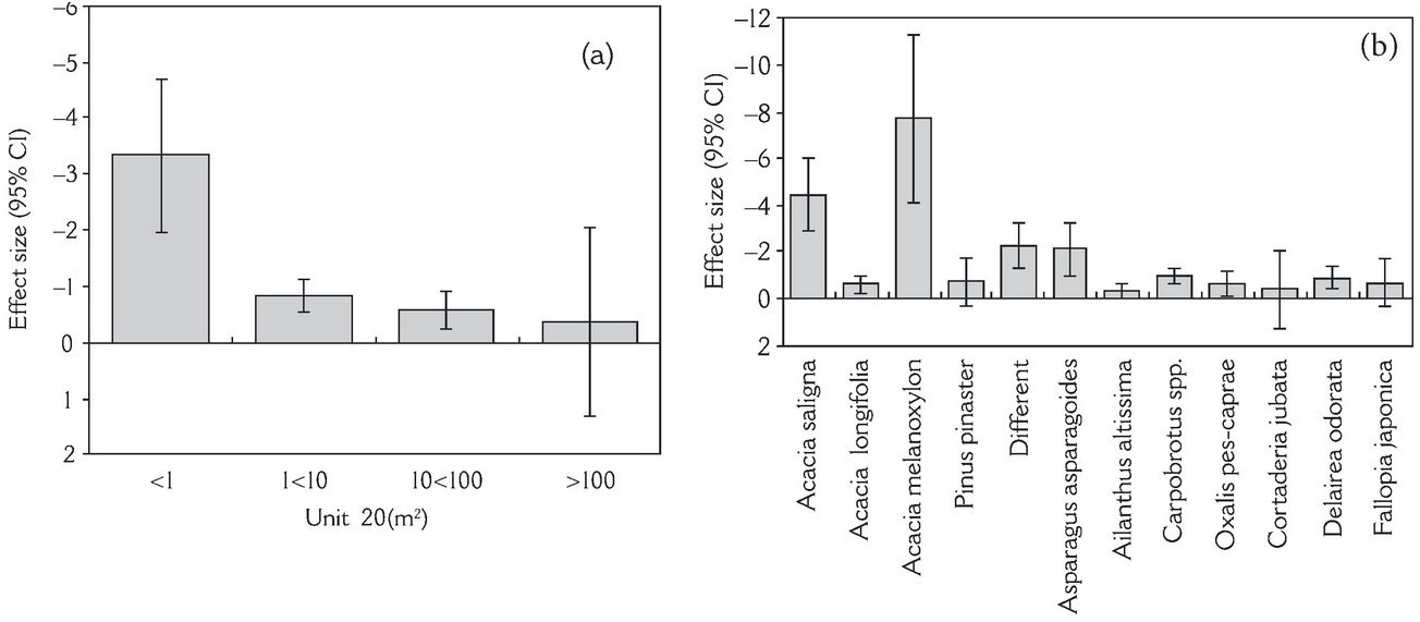
Figure 1.4 Effect size (95% Cl) of invasion on species richness for different (a) unit sizes and (b) taxonomical groups in Mediterranean-type ecosystems. Q-test shows significant different effect sizes (heterogeneity) between unit sizes and between species.

From Gaertner et al. (2009), reproduced with permission.

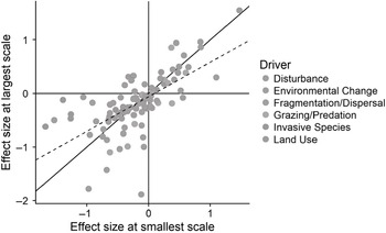
Figure 1.5 Results of a meta-analysis of scale-dependent responses to a number of different ecological drivers. Points represent the log response ratio comparing species richness in control to treatments in a given comparison measured at the smallest (x-value) and largest (y-value) scale. The solid line indicates the 1:1 line expected if effect sizes were not scale dependent. Points above and below this line indicate effect sizes that are larger or smaller, respectively, as scale increases; points in the upper left and lower right quadrants represent cases where the direction of change shifted from positive to negative, or vice versa, with increasing scale. The dashed line indicates the best fit correlation, which is significantly different than the 1:1 line (P < 0.01), indicating that overall, effect sizes tend to be larger at smaller scales than at larger scales. Colours for points indicate categorisations into different ecological drivers.

From Chase et al. (2018), reproduced with permission.

1.2 The Making of a Discipline

Although the human-mediated translocation of species has been documented anecdotally since antiquity, the concept of biological invasions is a very recent construct. Many naturalists in the 1800s wrote of non-native species, but it was only in the mid-1900s that the scale of human-mediated movements of species and the growing importance of the implications of such movement became apparent. Pioneers of ecology in the nineteenth century – among them Charles Darwin, Augustin and his son Alphonse de Candolle, Joseph Dalton Hooker and Charles Lyell – explored the role and performance of a small number of non-native species in competition with indigenous ones. Lyell (1832) wrote,

every species which has spread itself from a small point over a wide area, must, in like manner, have marked its progress by the diminution, or entire extirpation, of some other, and must maintain its ground by a successful struggle against the encroachments of other plants and animals.

Such appreciation of invasive spread leading to species extinctions predates the rise of global change biology in the late twentieth century (Wilkinson 2002). When writing about the European thistle cardoon, Cynara cardunculus, in his journal of research into the geology and natural history of the various countries visited by HMS Beagle, Darwin (1839) commented,

I doubt whether any case is on record, of an invasion on so grand a scale of one plant over the aborigines [of South America].

Following these early accounts of non-native species, many ecologists in the early twentieth century began synthesising the scattered knowledge of the ecology of non-natives, unknowingly taking the first tentative steps towards creating a framework for conceptualising biological invasions. Albert Thellung, in his 1912 Habilitation thesis La Flore Adventice de Montpellier, offered an early population-based definition of naturalisation which implied the notion of penetration of environmental barriers. He also devised concepts to classify the non-native flora of Montpellier in France according to their degree of naturalisation, introduction pathways and residence time (Kowarik and Pyšek 2012). Unfortunately, such work did not have much, if any, influence on the emerging field of ecology, and the ideas were only rediscovered in the late twentieth century, as the underpinning concepts of invasion science began coming under intense scrutiny.

Charles Elton’s (1958) classic book The Ecology of Invasions by Animals and Plants is recognised as a milestone in the development of the field now known as invasion science (Richardson and Pyšek 2007, 2008). Already expressed in Elton’s (1927) book on Animal Ecology, the Eltonian niche is an important concept for formulating a species’ position in an ecological network using its functional traits, as will be elaborated in later chapters. Following this line of thinking, Elton (1958) speculated that island assemblages are filtered for a small portion of colonisers, which subsequently cannot fully explore the island’s resources and are therefore more susceptible to invasions than those on the mainland. However, the publication of Elton’s book was not immediately followed by a significant rallying of research effort. Unlike some other books on environmental topics, Elton’s book on invasions had a negligible impact on public perceptions and launched no major actions (Hobbs and Richardson 2010). At about the same time as Elton’s book appeared, geneticists began synthesising concepts pertaining to the evolution and genetics of colonising species (Baker and Stebbins 1965). These insights provided crucial stepping stones to the development of the central tenets of invasion science, including the determinants of invasion success, life-history trade-offs, generalist versus specialist strategies, general-purpose genotypes, adaptive phenotypic plasticity, mating systems and the influence of bottlenecks on genetic variation (Barrett 2015). Perhaps the most important linkage of Elton’s (1958) classic volume to the theme of our book is his notion that decreased diversity leads to decreased stability. This complexity–stability relationship has stimulated long-lasting debates in ecology with substantial inputs from many figures in the field, including Robert MacArthur, Robert May and G. Evelyn Hutchinson. As will be shown in Chapter 4, ecological networks facing biological invasions typically violate this relationship but simultaneously reveal their trajectory of transition and turnover.

In 1980, the third international conference on mediterranean-type ecosystems, termed MEDECOS, was held in Stellenbosch, South Africa. The invasion of fynbos vegetation by non-native trees, a prominent topic of discussion at this meeting, conflicted with the dominant view of the time, which was that human-induced disturbance was the prerequisite for invasion into pristine ecosystems. A proposal drafted at the Stellenbosch meeting led to an international programme on the ecology of biological invasions under the auspices of the Scientific Committee on Problems of the Environment (SCOPE) (Mooney 1998). Its first five-year plan (1982–1986) revisited Elton’s key assumptions and generalisations, reviewed the status of invasions worldwide and addressed three key questions relating to invasiveness, invasibility and management. The SCOPE programme attracted some of the world’s top ecologists and comprised national, regional and thematic groups covering all aspects of invasions (Drake et al. 1989). Through the SCOPE programme, invasion science has firmly established itself as an exciting and relevant research field within global change biology (Simberloff 2011). In 1996, an influential conference in Trondheim, Norway, concluded that invasions had become one of the most significant threats to global biodiversity and called for a global strategy to address the problem (Mooney 1999; Sandlund et al. 1999). This led to the launch of the Global Invasive Species Programme (GISP Phase 1) in 1997, with more transdisciplinary goals than the SCOPE programme, acknowledging the need for work on economic valuation, stakeholder participation and pathway analysis and management (Mooney et al. 2005). The Convention on Biological Diversity (CBD), Article 8(h), calls on member governments to control, eradicate or prevent the introduction of those non-native species that threaten ecosystems, habitats or species. In 2000, the IUCN published their guidelines for the prevention of biodiversity loss caused by non-native invasive species. The 1990s saw the blossoming of invasion science, with the number of publications growing rapidly in all related fields (Vaz et al. 2017). In 2018 the Intergovernmental Science-Policy Platform on Biodiversity and Ecosystem Services (IPBES) launched a thematic assessment of invasive non-native species and their control.

Invasion science, as is the case with any emerging discipline, has exhibited different phases. From 1950 to 1990, studies on biological invasions were rather sparse, with fewer than ten publications per year according to the ISI Web of Science. In 1999, the journal Biological Invasions was launched, with its founding editor James T. Carlton (1999) stating,

[the aim of] Biological Invasions [the journal] … is to seek the threads that bind for an evolutionary and ecological understanding of invasions across terrestrial, fresh water, and salt water environments. Specifically, we [the journal] offer a portal for research on the patterns and processes of invasions across the broadest menu: the ecological consequences of invasions as they are deduced by experimentation, the factors that influence transport, inoculation, establishment, and persistence of non-native species, the mechanisms that control the abundance and distribution of invasions, and the genetic consequences of invasions.

The period 1990 to 2010 saw the rapid rise of invasion science and its multidisciplinary tentacles (Richardson et al. 2011; Vaz et al. 2017). During this phase, competing concepts, hypotheses, models and knowledge frameworks have been proposed and debated, and consensus has been reached on many fronts; we call this ‘Invasion Science 1.0’. Knowledge systems developed during this period accumulated mainly through individual case studies and comparative studies, with the focus being on the invader itself. Developments in the study of invasions at this time must be considered within the context of the intellectual landscape of the day. Indeed, following the Clements–Gleason debate, the Gleasonian individualistic notion that species function independently from the influence of others was implicitly accepted by most researchers as the foundation on which to build frameworks and concepts about ecological communities (Mascaro et al. 2013). As a result, Invasion Science 1.0 sought synergies mainly with population ecology, initially, and macroecology, more recently. The toolbox assimilated via this route served the field reasonably well, until problems began emerging early in the new millennium. As detailed later in this chapter, the growing frustration from contextual complexity and the lack of genuine predictability in invasion science, tentatively due to Gleason’s individualistic view, has driven many to search for alternatives, especially with the rise of network science, and call for the synergy between invasion science and community and network ecology; we call this ‘Invasion Science 2.0’ – the focus of this book. To start off, however, we use the rest of this chapter to delve into Invasion Science 1.0 and discuss its key concepts, achievements and shortcomings.

1.3 A Unified Invasion Framework

With the flourishing of invasion science in the new millennium, a number of frameworks emerged that were grasped by researchers to guide research on the ecology and management of invasions (Wilson et al. 2020a). Several protocols were proposed to synthesise the current understanding of invasiveness and invasibility into simple flow-chart models for assessing the risk of newly introduced species becoming invasive. The Australian Weed Assessment scheme (originally proposed by Pheloung et al. 1999) has been the most widely applied of these protocols. Phase 2 of GISP (2006–2010) set out to improve the scientific basis for decision-making to enhance the ability to manage invasive species; assess the impacts of invasions on major economic sectors; and create a supportive environment for the improved management of invasions. This initiative stimulated many new directions in research to elucidate the multiple dimensions of the impacts of invasive species and to utilise existing knowledge and incorporate new ideas and methodologies to inform options for management (e.g., Richardson et al. 2000; Clout and Williams 2009; Wilson et al. 2017). Substantial progress was made towards deriving general models of invasion, such as the ‘unified framework for biological invasions’ (Blackburn et al. 2011), which sought to merge insights from many previous attempts to conceptualise key aspects of invasion dynamics for all taxa (Figure 1.6; Table 1.1). This model, reinforcing the utility of conceptualising the many processes implicated in the phenomena of biological invasions using a series of barriers along an introduction–naturalisation–invasion continuum, has been widely applied (Wilson et al. 2020b). It provided an objective framework for linking theoretical and applied aspects in invasion science, and reinforced the foundations for a standard lexicon of terms for the field of invasion science (Richardson et al. 2011).

Figure 1.6 The unified framework for biological invasions. The framework recognizes that: the invasion process can be divided into a series of stages; that in each stage there are barriers that need to be overcome for a species or population to pass on to the next stage; that species are referred to by different terms depending on the stage in the invasion process they have reached; and that different management interventions are feasible at different stages. Different parts of this framework emphasise views of invasions that focus on individuals, populations, processes or species. The unfilled block arrows describe the movement of species along the invasion framework with respect to the barriers; alphanumeric codes associated with the arrows relate to the categorisation of species with respect to the invasion pathway given in Table 1.1.

From Blackburn et al. (2011); reproduced with permission.

Table 1.1 A categorisation scheme for populations in the unified framework of biological invasions. From Blackburn et al. (2011).

Category	Definition
A	Not transported beyond limits of native range
B1	Individuals transported beyond limits of native range, and in captivity or quarantine (i.e., individuals provided with conditions suitable for them, but explicit measures of containment are in place)
B2	Individuals transported beyond limits of native range, and in cultivation (i.e., individuals provided with conditions suitable for them but explicit measures to prevent dispersal are limited at best)
B3	Individuals transported beyond limits of native range, and directly released into novel environment
C0	Individuals released into the wild (i.e., outside of captivity or cultivation) in location where introduced, but incapable of surviving for a significant period
C1	Individuals surviving in the wild (i.e., outside of captivity or cultivation) in location where introduced, no reproduction
C2	Individuals surviving in the wild in location where introduced, reproduction occurring, but population not self-sustaining
C3	Individuals surviving in the wild in location where introduced, reproduction occurring and population self-sustaining
D1	Self-sustaining population in the wild, with individuals surviving a significant distance from the original point of introduction
D2	Self-sustaining population in the wild, with individuals surviving and reproducing a significant distance from the original point of introduction
E	Fully invasive species, with individuals dispersing, surviving and reproducing at multiple sites across a greater or lesser spectrum of habitats and extent of occurrence

1.4 Pathways and Propagules

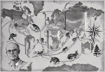
The premise of any biological invasion is the introduction of non-native propagules via invasion pathways that are required to breach ecological barriers and physical distance. Elton (1958) summarised his view in a chapter called ‘The Invasion of the Continents’, on pathways and the breakdown of geographic isolation through human-induced movement of organisms around the world. He likened the continents to great tanks of water, connected by narrow tubing blocked by taps. Using this analogy, he conceptualised the processes of biological invasions as interlinked tanks of propagule sources via introduction tubes (Figure 1.7),

Fill these tanks with different mixtures of a hundred thousand different chemical substances in solution… then turn on each tap for a minute each day… the substances would slowly diffuse from one tank to another. If the tubes were narrow and thousands of miles long, the process would be very slow. It might take quite a long time before the system came into final equilibrium, and when this happened a great many of the substances would have been recombined and, as specific compounds, disappeared from the mixture, with new ones from other tanks taking their places. The tanks are the continents, the tubes represent human transport along lines of commerce.

Figure 1.7 Elton’s vision of global biological invasions across continents via invasion pathways.

Artwork by Lorraine Blumer. Copyright: DSI-NRF Centre of Excellence for Invasion Biology. Reproduced with permission.

Six such introduction tubes, now known as invasion pathways, have been described (Table 1.2; Hulme et al. 2008) and adopted by the CBD. Invasion management targeting surveillance, mitigation and rapid response can efficiently target related invasion pathways and associated non-native taxa, before the species can gain foothold in new territories. Except for the unaided pathway of natural dispersal, the rest reflect clear management negligence and surveillance gaps that should be targeted by various different agencies (Hulme 2015). When combined with the unified framework (Section 1.3), biological invasions via different pathways were found to have different levels of invasion performance (Wilson et al. 2009). For instance, of those non-native plant species introduced to Central Europe, the pathways of release and contamination have resulted in higher than expected proportions of naturalised and invasive species, whereas the pathways of escape and stowaway do not (Pyšek et al. 2011). Each pathway also faces its own cataloguing issues as multiple pathways can be involved in one invasion, while the contribution of each pathway to non-native species introduction varies in terms of geographic, taxonomic and temporal contexts (Essl et al. 2015b). For example, the invasion of marine species in Western Europe is predominantly driven by shipping and aquaculture, whereas in the Eastern Mediterranean countries marine invasions are largely the result of the human-mediated opening of corridors, in this case largely the Suez Canal (Figure 1.8a). After WWII, aquaculture gradually declined as an important pathway for freshwater invasions, while the pathway through the pet trade, terrarium and aquarium is on the rise (Figure 1.8b). The release of non-native terrestrial arthropods for biocontrol was a reasonable practice in Europe until 2000 (green belt in Figure 1.8c), probably due to the implementation of the EPPO (European and Mediterranean Plant Protection Organization) standard in 1999.

Table 1.2 Six invasion pathways and related policy issues. Several key science and policy issues that should be considered if invasion pathways are to be successfully managed to prevent the introduction of invasive non-native species. From Hulme (2015) with modified examples.

Pathway	Example	Science issues	Policy issues
Release	The Asian Carp was introduced to the southern United States to clean commercial ponds in the 1970s but considered invasive by US FWS in 2006 and threatening the Great Lakes ecosystem.	Improved risk assessment tools to quantify the likelihood of economic, environmental and social impact of species with no prior history of introduction outside their native range.	Legislation that holds parties undertaking assisted colonisation responsible for any costs arising from the impacts and management of such introductions (e.g., assurance bonds).
Escape	Wild pet trade, for example, Burmese python Python bivittatus (Kuhl) in Florida.	Identify current commercial activities affecting risk management in the wild pet trade, reasons for non‐compliance and ways to change such behaviours.	Promote a whitelist approach to the trade in wild pet species, based on sound risk assessment yet also offering significant commercial benefits.
Contaminant	As a result of adult beetles or larvae hidden in wooden pallets on a ship, the Polyphagous Shot Hole Borer Euwallacea fornicatus is rapidly killing trees in South Africa by transmitting the fungus Fusarium euwallaceae.	Enhanced next‐generation DNA tools and biosystematic data to allow rapid screening of live commodities for cryptic pathogens and parasites.	Extend existing policies on risk prevention of emerging diseases to address the threats posed to biodiversity and ecosystem function.
Stowaway	Tourists might carry SARS-CoV-2 and cause the COVID-19 pandemic.	Analyse the risks from increasing tourist numbers, changes in countries of origin of tourists and shifts in location and types of tourism activities.	Robust codes of practice for tourism operators, aiming to prevent the introduction and movement of invasive non-native species.
Corridor	Canal development, for example, rabbitfish Siganus luridus introduced through Suez Canal.	Better prediction of the invaders that might be facilitated by corridors, the potential costs of future impacts and the value of practical measures to mitigate impacts.	International legislation to support environmental risk assessments of major infrastructure projects that include transboundary consequences.
Unaided	Lyme disease outbreak in Canada from bacteria Borrelia burgdorferi transmitted through bites by immature blacklegged ticks (the vector has extended its northern range potentially due to climate change).	New modelling tools to predict how wind and sea currents as well as extreme weather events can lead to long‐distance dispersal of non-native species.	Polluter pays principle applied where countries fail to contain or eradicate an invasive non-native species with potential to cause detrimental impacts should it spread beyond national borders.

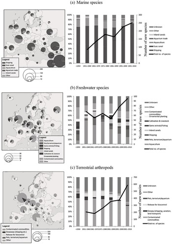
Figure 1.8 Geographic, taxonomic and temporal variation in the importance of the main pathways of introduction for non-native (a) marine species, (b) freshwater species or (c) terrestrial arthropods in Europe. The size of the pie charts indicates the approximate numbers of non-native species per recipient country of first introduction. Temporal trends of new introductions (the right panels) are given as black lines (the right axes). The pathway ‘Suez Canal’ (a) refers to Red Sea species that moved unaided into the Mediterranean via the Suez Canal.

From Essl et al. (2015b), reproduced with permission.

In reality, multiple pathways can facilitate invasions from different source areas at different stages, while propagules are transferred through these pathways at different rates and times in different contexts. This web of pathways facilitates recurrent bridgehead effects of invasions and gives rise to a pathway network. For instance, three quarters of the non-native ant species intercepted by US air and maritime ports between 1914 and 2013 are from countries into which the species were previously introduced, via similar or other pathways from its native range (Figure 1.9; Bertelsmeier et al. 2018). This further increases the genetic diversity of the introduced species and potentially improves their invasion performance in their new homes. However, a fully-fledged Pathway Network Analysis for most types of biological invasions is still not feasible because of limited data availability and resolution problems. Comprehensive pathway network analyses are undertaken to trace disease-related, protein-coding genes with gene expression data; these analyses use powerful statistical approaches and software developed to identify critical pathways for drug design and disease treatment (Khatri et al. 2012). Such pathway network analyses may be feasible in invasion science when the field has fully embraced data science and informatics, and when new methods are in place to collect and manage large volumes of high-resolution data and geographic and taxonomic coverage at a pace relevant to management.

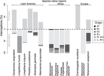
Figure 1.9 Percentage of primary v. secondary introductions of the most frequently intercepted ant species in the United States. The proportion of interceptions from the species’ native countries is shown above the x-axis (in grey) and the proportion of interceptions from countries in the non-native range below the x-axis (in colour). The colour code indicates the origin of the secondarily intercepted species. Species were visually grouped on the x-axis according to their native range (Dataset S1). Af, Africa; As, Asia; Eu, Europe; N. Am, North America; L. Am, Latin America; Oc, Oceania.

From Bertelsmeier et al. (2018); reproduced with permission.

The total number of non-native propagules introduced to an area through a pathway network, known as the propagule pressure (Lockwood et al. 2005), is the best-supported driver of invasion establishment and success. Although invasion performance is often caused by a chain of demographic actions (Gurevitch et al. 2011), early demographic advantage can provide a long-lasting boost to invasion dynamics, and often leaves an imprint on subsequent invasion dynamics (related to transient dynamics; Stott et al. 2011; Caswell 2019). Propagule pressure typically trumps any niche processes and filters imposed in the recipient ecosystems (Carr et al. 2019). According to a recent meta-analysis (Cassey et al. 2018), the relationship between propagule pressure and non-native population establishment success is consistently strong, showing a logistic form against the log-transformed propagule size (Figure 1.10). Such a saturation shape resembles the relationship between population viability and initial population size (McGraw and Furedi 2005), suggesting a mirror image between invasion and extinction (Figure 1.11; Colautti et al. 2017). As such, biological invasions are better formulated as an open and non-equilibrial system (Hui and Richardson 2019). Constant propagule influx is crucial to erase the genetic bottleneck anticipated for most invasive species as only a small sample of propagules are actually introduced (Simberloff 2009), although the impact of such obvious genetic bottlenecks on establishment might be weaker than previously thought because of rapid local adaptation (Dlugosch and Parker 2008).

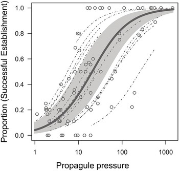
Figure 1.10 Estimated relationship of establishment success with propagule pressure and 95% credible interval (shaded). Dashed lines are individual experimental relationships based on a logistic model with random variation in the intercept and slope among individual experiments. Data points are raw data from 14 relationships from 11 studies that experimentally tested associations between propagule pressure and establishment probability.

From Cassey et al. (2018), under CC-BY Licence.

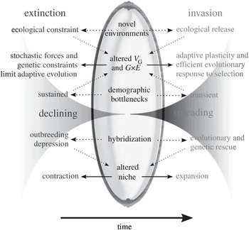
Figure 1.11 Extinctions and invasions conceptualised ‘Through the Looking Glass’ of evolutionary ecology. Extinctions (left side) represent population decline over time, while biological invasions (right side) represent an increase in abundance. Both invasions and extinctions reflect a common set of elements (central column) because subtle but influential ecological and genetic differences (outer columns) can cause opposite population growth trajectories.

From Colautti et al. (2017), reproduced with permission.

1.5 Invasion Dynamics

With invasion pathways and propagule pressure clarified, many researchers have focused their efforts on investigating the behaviour and mechanisms underlying the diverse forms of invasion dynamics. Invasion dynamics are highly stochastic and context dependent, making attempts to synthesise knowledge and predict particular cases challenging to say the least (Pyšek et al 2020b). This is not only a result of the spatiotemporal complexity of any given ecosystems but also the stochastic nature of invasive spread itself. The two demographic processes involved in spreading – growth and dispersal – both contribute to demographic stochasticity and contextual dependence (Hui et al. 2011b). Demographic rates such as the population growth rate of an invader can be scale-dependent and often exhibit specific spatial covariance structures in the invaded range (Gurevitch et al. 2016; Hui et al. 2017). The dispersal of an invader, often depicted as the dispersal kernel (probability distribution of dispersal distance), can also be anisotropic and reflect context-dependent movement strategies (e.g., good-stay, bad-disperse dispersal behaviour; Hui et al. 2012). The availability of natural enemies and dispersal barriers, as well as the novel ecological and evolutionary experiences facing each non-native organism (Schittko et al. 2020), make each turn a decision that affects the future possibilities of its invasion performance and dynamics. For instance, in the early 1900s when acclimatisation societies introduced the common starling, Sturnus vulgaris, into North America, southeastern Australia and the Western Cape of South Africa, the different propagule pressures, geographies and climates of the three regions resulted in distinct rates and directions of invasive spread across the three regions (Okubo 1980: Phair et al. 2018). Despite such challenges, progress has been made that allows us to grasp the processes and mechanisms behind a plethora of invasion dynamics (Hui and Richardson 2017). Here we highlight only a few aspects that are especially relevant to later chapters.

Once geographic barriers have been breached, via human facilitation, non-native organisms embark on their invasion and spread in recipient ecosystems. Patterns of invasion dynamics are diverse but can be summarised into different types for convenience (Hui and Richardson 2017), although the reality is much fuzzier around these thematic curves. Essentially, invasion dynamics can be divided into transient and asymptotic phases, where the former is highly flexible but the latter more consistent, reflecting the potential within a given habitat (see invasion curves in Figure 1.12a). In the invasion science literature, the curve of a specific invasion is often found to have multiple phases (Figure 1.12b), with a lag phase after introduction and before invasive expansion, and a biphasic range expansion of a slow phase followed by a fast phase. Over a longer period, the trajectory resembles a logistic curve and can be divided into acceleration and saturation phases (Figure 1.12c). For some invaders, success is transient, and its population size may follow a boom-and-bust trajectory, eventually settling at a much lower level, while the invaded range can percolate back from a continuous range to multiple smaller scattered local populations (Figure 1.12d). Such diverse forms of invasion dynamics – the duration, timing and speed of different phases – can be explained by different constraints and limiting factors through the invader constantly experiencing and exploring the novel environment in its invaded range, not only behaviourally by individuals of the non-native species but also ecologically and evolutionarily by its niche dynamics.

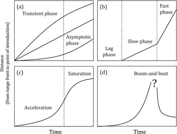
Figure 1.12 A variety of possible invasion dynamics. The invasion expansion of a non-native species is often documented as the distance from the advancing range front to the point of introduction over time. (a) Invasion dynamics are divided into two phases: a transient phase that is highly context-dependent which converges gradually to an asymptotic phase during which spread occurs at constant velocity. (b) Invasion dynamics are divided into a lag phase (no expansion for a period after introduction), and then slow and fast phases during which expansion occurs at a constant velocity. (c) A typical logistic curve for highly mobile species with an acceleration phase and a saturation phase as invasible space is occupied. (d) Boom-and-bust invasions are often caused by the collapse of local demographic processes, or by the encounter of an efficient natural enemy that has switched to target the non-native resource species when the non-native resource reaches an abundance threshold.

In terms of spreading dynamics, physicists and modellers have made great strides in elucidating the phenomenon of particle diffusion and dispersion in a suspension matrix. The Brownian movement of pollen grains in water, driven by the collision of numerous water molecules and the pollen, has enjoyed the attention of many renowned physicists, including Albert Einstein (1905). Collectively, such random movements of particles can be studied using specific models of partial differential equations known as reaction–diffusion models. Adolf Eugen Fick (1829–1901) described two laws of diffusion in 1855. Fick’s first law relates the diffusive flux to the concentration, assuming a steady state (Fick 1855). It postulates that the flux goes from regions of high concentration to regions of low concentration, with a magnitude proportional to the concentration gradient (i.e., spatial derivative); in simplistic terms, a solute moves from a region of high concentration to a region of low concentration across a concentration gradient. Fick’s second law predicts how diffusion causes the concentration to change with respect to time. Based on Fick’s second law, Ronald Fisher (1937) developed the now famous reaction–diffusion model which depicts the advancing wave of advantageous genes in the context of population dynamics

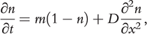$\frac{\partial n}{\partial t}=\mathrm{rn}\left(1-n\right)+D\frac{{\partial }^{2}n}{\partial x^2},$(1.1)

where $n$ represents the population density and is a function of time $t$ and location $x$ (thus more explicitly, $n\left(t,x\right)$). The left of this equation describes the time derivative of population density. The first term on the right depicts a simple logistic growth, with $r$ reactivity (here, the intrinsic rate of growth). The second term on the right depicts diffusion as a second order derivative of population density over space, known as the Laplacian operator; this term describes how uneven population densities (i.e., density gradients) in a local area are smoothed out. The diffusion cannot even out constant gradients of densities (e.g., at the range front), and consequently propels the population to spread along the direction of the gradient, forming a travelling wave. Fisher (1937) derived the travelling wave solution of the system. He concluded that the spreading velocity ‘is proportional to the square root of the intensity of selective advantage [$r$] and to the standard deviation of scattering in each generation [$\sigma$]’, as $v=\sigma \sqrt{2r}$, or ‘equivalently to the square root of the diffusion coefficient when time is measured in generation’, as $v=2\sqrt{\mathrm{rD}}$. This milestone not only provides a way to estimate the diffusion rate based on movement records (e.g., from ringing and mark-recapture data) as $D={\sigma }^2/2$ but also derives a commonly used estimate of spreading velocity that has been the backbone of many models of spread ever since. A classic example is by Okubo (1980) who used this model to explore the invasive spread of common starlings, Sturnus vulgaris, in North America. This has resulted in such developments as velocity estimates under biotic interactions, density dependence (e.g., Allee effect), heterogeneous habitats, drift/convection in environments and biotic interactions (see review by Hui et al. 2011b).

A major challenge facing diffusion-type models is related to Reid’s (1899) paradox of rapid northward plant migration after the last glacial maximum. In Reid’s words, ‘the oak, to gain its present most northerly position in northern Britain after being driven out by the cold, probably had to travel fully six hundred miles, and this, without external aid, would take something like a million years’ (see updated review by Davis and Shaw 2001; Figure 1.13). This is probabilistically impossible when estimated based on $r$ and $D$ measured for today’s oak populations, while the unrealistically high levels of population growth rate and diffusion rate suggest alternatives (Skellam 1951). The inability of reaction–diffusion models to accommodate Reid’s paradox has led to a systematic shift in paleoecology away from the use of population ecology models that partition observed velocity into demographic factors of population growth and dispersal in driving such range shifts (Clark et al. 1998).

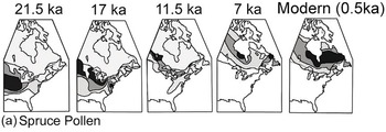
(a) Spruce pollen representing three extant species plus the extinct P. critchfieldii. More recent data show that spruce was abundant further south in the Mississippi valley during the Last Glacial Maximum than shown here. Both southern and northern range boundaries of spruce shifted northward.

(b) Oak pollen representing some or all of the 27 extant Quercus species in eastern North America. Oak expanded from the southeast but continued to grow near locations of full-glacial refuges.

From Davis and Shaw (2001); reproduced with permission.

Figure 1.13 Ranges, as indicated by pollen percentages in sediment, of spruce (Picea) and oak (Quercus) in eastern North America at intervals during the late Quaternary. The continental ice sheet is shown in blue; pollen proportions are shown in shades of green. The shoreline is not drawn to reflect changes in sea level.

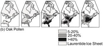
Two mechanisms have received substantial support in invasion science for explaining such an augmented spreading velocity, as anticipated by Reid’s paradox. First, the forms of dispersal kernels can be diverse. While the standard deviation of dispersal distances is only a representative shape metric for Gaussian-type kernels, it fails to capture the ‘average’ for highly skewed, often fat-tailed, dispersal kernels. For instance, extremely rare dispersal events of non-native species over large distances can occur, often mediated by human activities that skew the dispersal kernel (e.g., Suarez et al. 2001). To accommodate rare long-distance dispersal events, models with stratified dispersal kernels (i.e., a combination of different modes of dispersal) have been proposed, especially to explain biphasic range expansion (Figure 1.12b; Shigesada and Kawasaki 1995). More explicit modelling, however, needs to implement realistic dispersal kernels directly. This can be handled flexibly by using integral equations. Integral equations have a long history in mathematics (Fredholm 1903); they were first applied in invasion ecology by Van den Bosch (1992) and Kot et al. (1996). A generic form of an integrodifference equation is

$n\left(x,t+1\right)=\int k\left(x,y\right)f\left(n\left(y,t\right)\right)n\left(y,t\right)\mathrm{dy}.$(1.2)

where the population density $n\left(x,t+1\right)$ at time $t+1$ in location $x$ can be calculated as the integral (or the summation) of propagules from all possible locations in the previous time step $n\left(y,t\right)$ multiplied by the per-capita population growth rate during one time step $f\left(n\left(y,t\right)\right)$, and weighted by the dispersal kernel $k\left(x,y\right)$ that depicts the chance of a propagule moving from location $y$ to location $x$ within one time step. A vector format of such equations is easily extended to accommodate population structures of species with complex life-cycles and life stage-dependent dispersal modes. In such models, dispersal kernels are typically implemented as only distance dependent $k\left(d\right)$, with the distance $d=\left(x-y\right)$, while more realistic movement can be captured directly by considering explicitly the beginning and end locations, $y$ and $x$ respectively. One important way to boost up the rate of spread comes with the realisation that the movement of most organisms, especially those that disperse via means other than gravity, follows the pattern of Lévy flights (e.g., $k\left(d\right)~d^{-3/2}$ in Figure 1.14 for the common starling). Unlike Gaussian-type kernels with finite mean and variance, such a power-law dispersal kernel is of infinite variance, meaning that the movement can have diverse characteristic length, and is highly flexible to handle complex and novel context. A power law dispersal kernel could reflect that the movements of individuals are self-organised near criticality that enables the species to cover novel and heterogeneous resource landscapes with maximum flexibility and minimum energy input (Muñoz 2018).

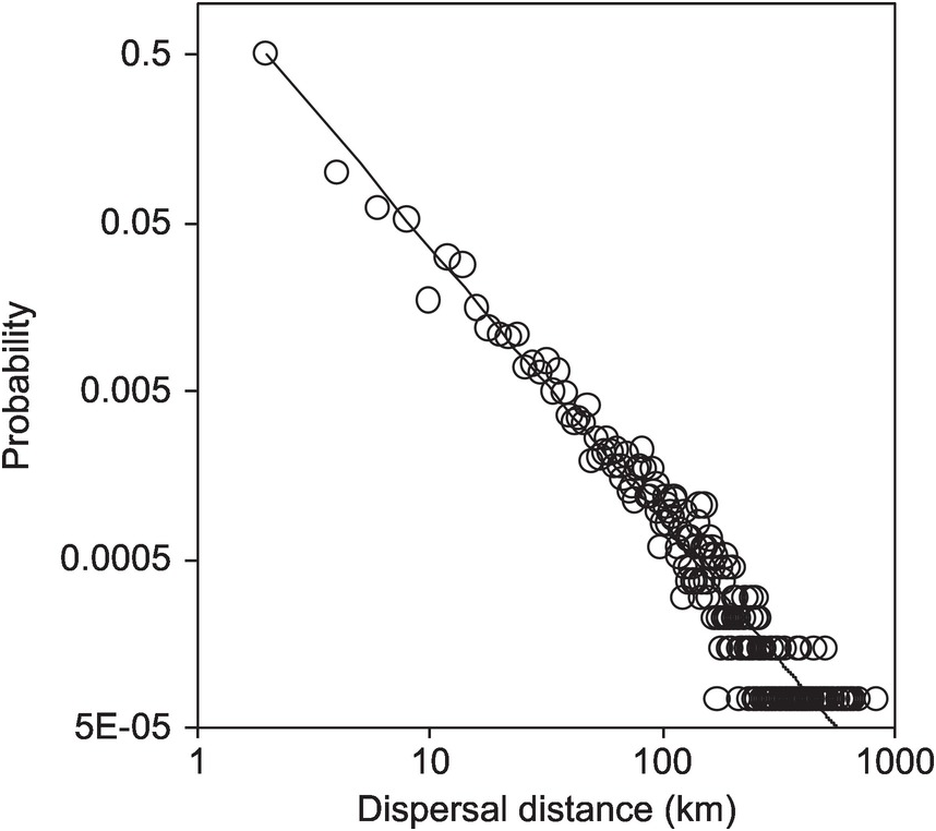
Figure 1.14 The inverse power function of the dispersal kernel for all movements of European starling Sturnus vulgaris within Britain during the breeding season. Dispersal kernels are produced using a 2 km distance class; that is, all records are binned to the dispersal distance class of < 2 km, 2–4 km, 4–6 km, and so on.

From Hui et al. (2012); reproduced with permission.

Second, spatial sorting has emerged as a clear pattern in many invasive species when comparing individuals from the core/introduction versus the periphery/front populations (Shine et al. 2011). The invasion of cane toads (Rhinella marina) in Australia provides the textbook example of spatial sorting in invasion ecology (Figure 1.15). This species was (imprudently, with the benefit of hindsight) introduced to Australia to control insect pests in sugar-cane fields. The annual rate of progress of the toad invasion front has increased fivefold since its introduction, with toads at the front having longer legs and moving faster (Phillips et al. 2006). The invasion of the common mynah (Acridotheris tristis) in South Africa also exhibited a clear pattern of spatial sorting. Dispersal-related traits such as wing-loading and length were clearly sorted along the distance to the introduction point, while foraging traits such as the ratio of bill length to width corresponded more to local habitat quality (Berthouly-Salazar et al. 2012). Spatial sorting is driven by both the non-equilibrium dynamics (ongoing advancing front) that continuously sieve out the front runners, and the declining density gradient (and thus the diminishing intensity of resource competition and increasing difficulty of finding a mate) from the core to the expansion front. These processes create two selection forces: (i) ‘first come first served’ that favours individuals with high dispersal ability, as well as those that are more aggressive and competitive; (ii) the low density at the range front further allows these individuals to possess higher fitness, thus creating the phenomenon of spatial sorting and spatial selection when range expansion is ongoing (Shine et al. 2011). The forces combined can create synergies to obviate the trade-off between dispersal and the cost of reproduction remedies to low densities (e.g., selfing), giving rise to the Good Coloniser Syndrome (Cheptou and Massol 2009; Rodger et al. 2018), as postulated by Baker (1955).

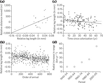
Figure 1.15 Morphology of cane toads (Rhinella marina) in relation to their speed and invasion history. (a and b) Compared with their shorter-legged conspecifics, cane toads with longer hind limbs move further over 3-day periods (r² = 0.34) (a), and are in the vanguard of the invasion front (based on order of arrival at the study site; r² = 0.11) (b). (c) Cane toads are relatively long-legged in recent populations, and show a significant decline in relative leg length with time in older populations (r² = 0.05). (d) The rate at which the toad invasion has progressed through tropical Australia has increased substantially since toads were first introduced in 1935 (r² = 0.92).

From Phillips et al. (2006); reproduced with permission.

When we consider a skewed dispersal kernel and spatial sorting of propagules with different dispersal capacities, we can derive an estimate of spreading velocity using integrodifference equations (Ramanantoanina et al. 2014)

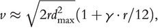$v\approx \sqrt{2{\mathrm{rd}}_{\max }^2}\left(1+\gamma \cdot r/12\right),$(1.3)

where $d_{\max }^2=exp\left(\mu +\sqrt{2{\sigma }^2}{erf}^{-1}\left(2^{1-1/n_0}-1\right)\right)$ represents the maximal dispersal ability in the non-native population, assuming the dispersal ability follows a lognormal distribution with $\mu$ and ${\sigma }^2$ its logarithmic mean and variance, and ${erf}^{-1}\left(\cdot \right)$ the inverse Gaussian error function; note, $n_0$ represents the initial propagule pressure, while $\gamma$ is the kurtosis of the dispersal kernel (a measure of second-order skewness). In short, the intrinsic population growth rate ($r$), the initial propagule pressure ($n_0$) and diversity ($\sigma$), as well as the degree of skewness of the dispersal kernel ($\gamma$), can all contribute positively to the spreading velocity of a non-native species.

Besides these overall explanations of the largely accelerated speed of invasion dynamics, it is important to consider context dependence. Not only do different non-native species exhibit different dynamics, but the same species can also have drastically different invasion velocities and follow different archetypes of invasion dynamics at different localities. Even in controlled environments, arguably under identical settings, the same species do not necessarily replicate their own invasion dynamics (Melbourne and Hastings 2012). Invasive species subject to Allee effects can exhibit invasion dynamics that are completely dependent on initial conditions; they can exhibit a whole spectrum of performance levels, from range pinning with stalled range expansion to high-speed range expansion (Keitt et al. 2001; Hui and Li 2006). We need to change our perspectives so to make sense of such a plethora of invasion dynamics scenarios. Think of a car. It can be driven in many ways: at high speed or low speed, with the engine revving fast, idling or stalling; it is impossible to summarise or predict how a car can be driven. However, to achieve a high speed, the way the clutch changes in a gearbox follows the same procedure, to balance the force (impact) and the speed by sequentially moving up the gears. Too high or too low a gear for a given speed can stall or burn the engine, respectively (Figure 1.16). The population structure of any species can be complex. Such complex, multistage life-cycles create a demographic transition matrix that propels the population dynamics. Demographic and dispersal rates of this ‘population engine’ are not constant, but depend on how the gear of population structures and densities of different life stages fits the engine of the demographic transition matrix, while driving along a heterogeneous terrain. During the functioning of this engine and to complete the life-cycle efficiently, particular vital rates become the limiting factor and control the gear. This can normally be revealed by exploring the dominant eigenvector(s) of the transition matrix, and the abundance vector of different life stages. When the abundance vector and the dominant eigenvector are aligned, they function like a perfect gear to maintain and boost speed. Shifting the dominant eigenvector will require a change of gear (abundance vector) to match up. So, to merge the diverse forms of invasion dynamics, we need to examine the engine and gearbox of biological invasions, and pay less attention to the dash-cam footages of particular journeys.

Figure 1.16 A schematic procedure of clutch changes in a gearbox to reach top speed. Each solid polynomial curve represents the performance of a particular gear (performance is depicted here as impact and velocity). A single gear cannot cover all the impact and velocity ranges. To speed up from standing still, we need to sequentially move up through the gears to avoid engine failure. The system can fail in two ways: high gear and low speed, or low gear and high speed. In species with complex life-cycles, different demographic rates serve as different gears (limiting factors) during invasion. Diverse invasion dynamics are therefore anticipated (see, for species with complex life-cycles, Figure 1.12).

1.6 Invasiveness and Invasion Syndromes

The invasiveness of a non-native species reflects directly its demographic performance (growth and dispersal), while multiple ecological and evolutionary processes are at play, forming a causal pathway network in determining the demographic performance of an invader (Figure 1.17; Gurevitch et al. 2011). In this causal pathway network, each arrow can be switched on and off, or set flickering to become stronger or weaker in a specific context, giving rise to a contextually realised causal pathway network behind the demographic performance of a particular non-native species. Some of these processes are directly related to invasiveness, while others indirectly affect invasiveness via mediators. We select a few factors that have been considered proxies of invasiveness: invasive traits, range size, dispersal strategies, spatial covariance and a trio platform of trait–site–pathway, which can explain invasion performance of a non-native species.

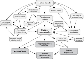
Figure 1.17 A conceptual synthetic invasion meta‐framework based on fundamental ecological and evolutionary processes and states. The three different characteristics of invasions and their effect on altering communities and landscapes are in bold capital letters. Transitions between the processes and states are indicated by arrows. Components found in more than one position affect or are affected by more than one set of other processes.

From Gurevitch et al. (2011); reproduced with permission.

There has been a long tradition of using comparative methods to identify invasive traits that can help pinpoint the propensity of a non-native species for invasion success (Van Kleunen et al. 2010a). A meta-analysis of trait differences between 125 invasive plant species and 196 paired non-invasive species in the invaded range revealed a number of consistent results (Van Kleunen et al. 2010b): after traits were grouped by physiology, leaf-area allocation, shoot allocation, growth rate, size and fitness, invasive species were found to have significantly higher values than non‐invasive species for all six trait categories (Figure 1.18a). Although trait differences were more pronounced between invasive and native species than between invasive and non‐invasive alien species (Figure 1.18b), comparisons between invasive species and native species which were invasive elsewhere yielded no significant trait differences (Figure 1.18c). Differences in physiology and growth rate were larger in tropical regions than in temperate regions (Figure 1.18d–f). Trait differences did not depend on whether the invasive non-native species originated from Europe, nor did they depend on the test environment (Figure 1.18g and h). More importantly, several studies have suggested that successful non-native species possess more distinct traits when compared to those native species in the community (e.g., Divíšek et al. 2018; Mathakutha et al. 2019), and such elevated invasion success could correspond to biotic novelty (Schittko et al. 2020). Trait distinctiveness and novelty relate more to how a non-native species takes advantage of empty niches available in an ecological network; we dive deeper into this topic in subsequent chapters.

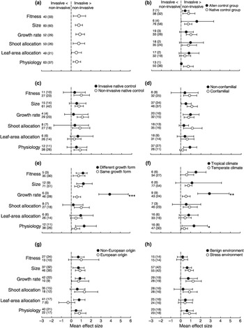
Figure 1.18 Mean effect sizes of differences between invasive non-native plant species and non‐invasive plant species for: (a) the six trait categories, and the dependency of these mean effect sizes on (b), whether the control species was a non‐invasive non-native species or a native species; (c) whether the native control species is known to be invasive elsewhere; (d) whether the invasive non-native species and non‐invasive species belong to the same family; (e) whether the invasive non-native species and non‐invasive species have the same growth form; (f) whether the study was performed in a temperate region or in a (sub)tropical region; (g) whether the invasive non-native species is native to Europe; and (h) whether the species were compared under benign environmental conditions or under more stressful environmental conditions. The bars around the means denote bias‐corrected 95% bootstrap‐confidence intervals. A mean effect size is significantly different from zero when its 95% confidence interval does not include zero. The sample sizes (i.e., number of species comparisons) and, in parentheses, the numbers of studies are given on the left‐hand side of each graph. Positive mean effect sizes indicate that the invasive non-native species had larger trait values than the non‐invasive species. Significant differences between factor levels (see Appendix S3): * P < 0.05; ** P < 0.01; *** P < 0.001.

From van Kleunen et al. (2010b); reproduced with permission.

Can invasion performance mirror how a non-native species ‘behaves’ in its native range? If the home and away performances mirror each other, one could predict the non-native performance by monitoring performance in the native range (and perhaps also in other invaded ranges). This is exactly what a number of studies have suggested: they show the strong effects of a non-native species’ native geographic range on its non-native performance. One obviously needs to consider the habitat and disturbance similarity/overlap between the native and non-native ranges, which limits the performance due to obvious physiological constraints. In a cross-taxon study (Hayes and Barry 2008), when comparing the traits of introduced species vs. those of invasive species, only two species-level characteristics – taxon and geographic range size – were consistently associated with establishment success. However, when comparing the traits of introduced and native species, three species-level characteristics – geographic range size, leaf surface area and fertilisation system (monoecious, hermaphroditic or dioecious) – were consistently found to be significantly different, but only for plants. However, whether geographic range size reflects inherent invasiveness or just human preference in selecting species to move is debatable. For instance, unlike invasive Australian acacias, the native range size of invasive Australian eucalypts is not significantly greater than that of naturalised species (Figure 1.20). Intriguingly, the human preference for introducing species with larger ranges was much greater for acacias than for eucalypts, as the geometric mean range sizes of introduced, naturalised and invasive acacias are 2.04, 1.88 and 3.59 times those of eucalypts that had attained the same invasion status (introduced/naturalised/invasive) (Hui et al. 2011a; 2014). The selection preference of acacias during introduction is thus for species that can rapidly expand their range; in contrast, slow spreading eucalypts have been selected for dissemination. In other words, humans appear to have selected for highly invasive acacias but against introducing highly invasive eucalypts (Figure 1.19).

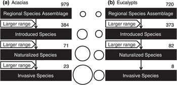
Figure 1.19 A schematic illustration of the selection bias of Australian (a) Acacia species and (b) eucalypts (genera Angophora, Eucalyptus and Corymbia) at different invasion stages for four cascaded lists. Only significant differences of native range sizes between two species lists are presented; differences in percolation intercept and exponent are not shown for conciseness. The number of species in each stage is indicated above each box. The circles between the boxes are proportional in area to the geometric mean range sizes of species in that stage.

From Hui et al. (2014); reproduced with permission.

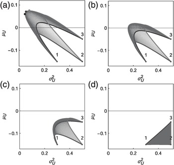
Figure 1.20 Expectation and variance of relative growth rate for an ensemble of three populations. Red, green and black curves: attainable sets for combinations of two populations. Blue mesh: attainable sets for combinations of three populations. Covariances between populations are the same in each plot and are calculated as the correlation multiplied by the standard deviations of the two populations. Correlation = −0.5 in (a), 0 in (b) representing independent; = 0.5 in (c); and = 1 in (d) representing perfect synchrony. The efficient frontier is calculated for the maximum growth portfolio (green dot in a), for the minimum variance portfolio (black dot in a) and for the portfolio on the efficient frontier where the attainable set is stretched the most along the ensemble shifting direction (purple dot in a).

From Hui et al. (2017); reproduced with permission.

Besides particular functional traits and species-level proxies that can tentatively explain species invasiveness, invasive performance has emerged as being highly context dependent. The results of invasive–native trait contrasts can be highly context dependent. When comparing resource-use traits in native and invasive plant species across eight diverse vegetation communities distributed across the world’s five Mediterranean climate regions, invasive traits differed strongly across regions (Funk et al. 2016). However, in regions with functional differences between native and invasive species groups, invasive species displayed traits consistent with high resource acquisition. The impacts of invasive species can also be highly context dependent. For instance, invasive plants exert consistently significant impacts on some outcomes (survival of resident biota, activity of resident animals, resident community productivity, mineral and nutrient content in plant tissues, and fire frequency and intensity), whereas for outcomes at the community level, such as species richness, diversity and soil resources, the significance of impacts is determined by interactions between species traits and the invaded biome (Pyšek et al. 2012). There is no universal measure of impact and the pattern observed depends on the ecological feature of interest. In short, the dynamics, performance and impact of an invasion are highly context dependent.

A potential explanation for this widely acknowledged context dependence is that successful invaders need to learn about their new environment and adapt to it, and therefore need to be flexible in heuristic learning. This generic learning can be achieved through a number of features – plasticity, rapid evolution or power-law dispersal (behaviour flexibility at criticality). For instance, invasive species are nearly always more plastic in their response to greater resource availability than non-invasive species, although this plasticity is not always correlated with a fitness gain. In other words, invasive species are more plastic in a variety of traits but non-invasive species respond just as well, if not better, when resources are limited (Davidson et al. 2011). Second, such a high level of context dependence is perhaps due to the rapid evolution anticipated in many introduced species (Whitney and Gabler 2008). Rapid evolutionary changes are common during invasions, perhaps as a result of new environments, effects of hybridisation and coevolution in recipient communities (Prentis et al. 2008). Typical invasion traits (e.g., growth rate, dispersal ability, generation time) can undergo evolutionary change following introduction over very short periods (e.g., within a decade). Rapid evolutionary change in many invasive species calls for added caution during risk assessment that often assumes a fixed life-history strategy in invaders. Finally, there could be a flexible learning strategy such as the ‘win-stay, lose-shift’ game strategy and the ‘good-stay, bad-disperse’ behaviour that could give rise to the power law dispersal kernel (Figure 1.14). A power-law dispersal kernel can emerge from self-organised movement of foragers when exploring a new heterogeneous resource landscape (Muñoz 2018). It can also give rise to specific spatial covariance between local population demographics, minimising population volatility but maximising population growth, such as those exhibited in the landscape demographics of the gypsy moth in the northeastern United States (Figure 1.20). Predicting invasive dynamics, performance and impacts under such extreme contextual dependence becomes ‘Mission: Impossible’.

Dealing with such highly context-dependent invasion performance, risk assessment and management has edged forwards by following a simplified three-pronged approach. Catford et al. (2009) summarised existing invasion hypotheses into three groups: those that involve propagule pressure, those that consider traits associated with invasiveness and those that deal with features of the environment that affect invasibility. Subsequently, invasion management has also been tasked with seeking balanced prioritisation by considering pathways, species traits and site characteristics (Figure 1.21a; McGeoch et al. 2016). The idea of a three-pronged approach has been further expanded by the concept of ‘invasion syndromes’ (Figure 1.21b; Novoa et al. 2020), where each of the trio – pathways, traits and sites – can be fine-tuned by invasion symptoms and contexts, and by our knowledge, from both the specific and generic. A specific invasion syndrome defines an archetype of invasion dynamics and impacts which can potentially be managed by applying a specific suite of policy and management actions. While the trio idea makes conceptual sense, the practicality of using this method is still questionable as most of the supporting cases are retrospective. Only with the accumulation of a large number of well-described cases will we be able to construct robust syndromes using a bottom-up approach with vigorous cross-validation. Well-described invasion cases and their management actions and consequences are only beginning to be systematically collected; it could require decades for such robust invasion syndromes with solid support to emerge.

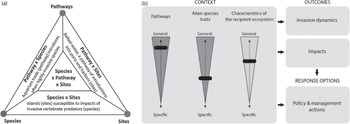
Figure 1.21 The three components of invasion syndromes (a) The three foci for a comprehensive approach to prioritising investment in management of biological invasions. Examples of combined prioritised risks associated with these focus areas, with the example in the centre being ornamental species in gardens as escapees (pathway) into adjacent protected areas (sites); From McGeoch et al. (2016); reproduced with permission. (b) An invasion syndrome is defined as a combination of pathways, non-native species traits and characteristics of the recipient ecosystem which collectively result in predictable dynamics and impacts, and which can be managed effectively using specific policy and management actions. For it to be coherent, the shared characteristics (pathways, non-native species traits and characteristics of the recipient ecosystem) must result in predictable outcomes (regarding invasion dynamics and impacts) which in turn can be best managed using similar management or policy responses. This means that invasion syndromes should be created from generalisations that are as broad as possible but which are still robust and useful. The invasion context is displayed here on three vertical axes (i.e., vertical black bars) that range from general (at the top) to specific (at the bottom). For example, the non-native species traits axis could vary (top/general to bottom/specific) from all aquatic species to aquatic species within a specific genus and to congeneric freshwater species within a specific body size range. The positions along the axes (i.e., black boxes) are adjusted so that all invasion events within the selected context result in similar outcomes and response options. A change in any one of the axes, or a change in the outcomes or response options that are to be encompassed by the invasion syndrome, will likely affect all other aspects of the framework, which means that circumscribing a syndrome is an iterative process.

From Novoa et al. (2020), under CC-BY Licence.

1.7 From Trees to Networks

Invasion Science 1.0 has followed an invader-centric view and has sought synergies from population ecology on the role of habitat quality and from demography in determining species performance. This species-centric view packages all factors that an invader needs to negotiate as eco-environmental barriers. What an invader confronts in its recipient ecosystem is not a passive pool of antagonists and resources that it has to contend with. Rather, all resident species and other socioeconomic components of the recipient ecosystem respond to the invasion simultaneously. The outcome of the invasion thus depends not only on the invader’s own strategies (behavioural, demographic, ecological, evolutionary) but also on the actions and strategies of all resident species and embedded components. This is a typical setting of game theory, where one player’s payoff not only depends on his/her own play but also that of its opponents. As Elton (1958) anticipated in his classic book

It is a very long haul from handling a small group of four species like the lemon tree, the nightshade, the black scale, and a chalcid parasite, to the contemplation of the most inconceivable and profuse richness of a tropical rain forest, or even to the several thousand species living in Wytham Woods, Berkshire. It is a question for future research, but an urgent one, how far one has to carry complexity in order to achieve any sort of equilibrium.

Indeed, we need to formulate the complexity of these ‘thousand species’ to achieve better understanding and predictability in invasion science. We think this can be done by nudging Invasion Science 1.0 and its synergies with population ecology towards Invasion Science 2.0, which embraces advances in community ecology, network ecology and ecosystem science. This does not require us to shift focus away from species but to expand it to allow for the critical inclusion of biotic interactions between and among species. It requires us to consider biological invasions in the context of ecological networks.

If we look again at the unified framework of invasion (Figure 1.6), the mother lode of Invasion Science 1.0, its linear and tree-like structure is obvious. Trees have been the metaphor for orderly and structured knowledge since antiquity, from the Tree of Life, genealogy, Aristotle’s taxonomic classification, to Darwin’s tentative sketch of a phylogeny. The barriers and stages of the invasion framework allow for structured response and prioritisations for targeting early stages for maximum interventions. However, these processes and barriers at different stages are intertwined and are species and context dependent. If we look at the current knowledge landscape in invasion science (Figure 1.22), we are faced with a complex network, comprising arguably five clusters (Enders et al. 2020). This landscape, of course, represents only the knowledge of invasion performance that has accumulated over the last few decades, mainly since 2000. More hypotheses and links, especially hyperlinks that simultaneously connect existing hypotheses, could emerge to drastically complicate or, oddly, simplify this congested landscape. Looking closely, we can see that the pathway–trait–site troika has been expanded here into pathway (propagule cluster), trait (trait cluster and Darwin’s cluster) and site (biotic interaction cluster and resource availability cluster). Although the resource availability cluster was positioned at the centre of this knowledge network, we put biotic interactions, more precisely ecological networks of biotic interactions, at the centre of subsequent chapters to highlight what we think is the key to understanding the complexity of biological invasions.

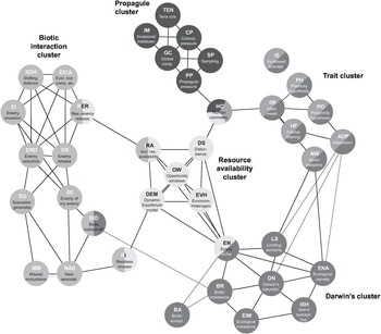
Figure 1.22 Network of 39 common hypotheses in invasion biology. Clusters were calculated using the local link-clustering algorithm. Colours indicate membership of hypotheses to concept clusters. The representation is simplified in that, for example, the node empty niche (EN) appears to be split into two equal parts, whereas it actually belongs slightly more to Darwin’s cluster (6/11 = 55%) than in the resource availability cluster (5/11 = 45%).

From Enders et al. (2020), under CC-BY Licence.

How many invasive species can our ecosystems tolerate? Human activities are intentionally and unintentionally introducing more and more species to new regions of the world – for example, via commodity transport or tourism. Some of these non-native species have negative consequences for biodiversity and human well-being, e.g., by displacing native species or transmitting diseases. However, while we have relatively good information on the historical spread of non-native species, there is still little knowledge on which to base predictions of future trends on invasion impacts. A poll of expert opinion suggests that an increase of 20 to 30 per cent in the number of newly introduced non-native species is considered sufficient to cause massive global biodiversity loss (Figure 1.23; Essl et al. 2020). Such an increase in the magnitude of invasions is likely to be reached soon, as the number of introduced species is constantly increasing. Furthermore, humans are the main drivers of the future spread of non-native species. The experts identified three main reasons: primarily the increase in the global transport of goods, followed by climate change and the extent of economic growth. The study also showed that the spread of non-native species can be greatly slowed down by ambitious countermeasures. Politicians have the responsibility to act.

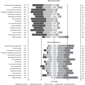
Figure 1.23 Distributions of uncertainty of 15 major drivers of biological invasions exhibit major impacts on the environment by 2050 under a best- and worst-case scenario, based on answers provided by 36 experts. The uncertainty categories follow a five-point Likert scale. The estimates shown include all responses across 14 contexts regarding taxonomic groups, zonobiomes, realms and socio-economic status. The stacked bars represent the uncertainty categories, with the bars and percentage value for the medium certain category centred at 0% on the x-axis. Bars and percentage values on the left refer to the uncertainty categories extremely and moderately uncertain, and bars and percentage values on the right refer to the answers in the categories highly and extremely certain. Categories sum up to 100%.

From Essl et al. (2020); reproduced with CC-BY Licence.

This daunting scientific and management challenge has led to authors labelling the management of some biological invasions a ‘wicked problem’ (Woodford et al. 2016). Indeed, the number of major success stories in the management of biological invasions is alarmingly small. The Aichi Biodiversity Target 9 states,

By 2020, invasive non-native species and pathways are identified and prioritised, priority species are controlled or eradicated, and measures are in place to manage pathways to prevent their introduction and establishment.

During the writing of this book in 2020, during the most dramatic phase of the invasion dynamics and impacts of COVID-19, it was clear that we have collectively failed to reach this target. The choice of a warlike word ‘invasion’ to describe this research field has been met with mixed sentiments. Many have vivid memories of reading stories of non-native invasions and the feelings associated with them as unfamiliar, strange or even scary, while invasion itself has been recorded throughout history as brutal and uncivilised, creating fear and sometimes irrational response. However, faced with global changes with multiple drivers that transform global ecosystems and the biosphere, fear is normal. If there is a way out of each crisis, perhaps we need to look attentively with fear and curiosity and see where the tides (and tsunamis) will take us. This fear and opportunity has driven some to deny, some to restore and some to leave the research field, and others to embrace the change as a whole new world of novel ecosystems. Even without using the warlike metaphor ‘invasion’, scientists in the field of global change are clearly loaded with fear and a slice of excitement. The pervasiveness of the current unprecedented global changes suggests that we can never turn back the clock to some bygone era. Instead, we need to steer or surf through the Volatility, Uncertainty, Complexity and Ambiguity (VUCA) wave of knowledge landscapes (Figure 1.24), transformed ecosystems and increasingly complex societal changes and responses. Of the four components of the VUCA diagram, the current agenda in invasion science is pushing the veiled line that divides Invasion Science 1.0 from Invasion Science 2.0 towards the top right. In Invasion Science 1.0, we have largely rooted out Ambiguity and are rapidly reducing Uncertainty by embracing informatics and data science, while we envisage embracing Complexity, and experiencing further Volatility in the knowledge enterprise of invasion science when it transitions to Invasion Science 2.0.

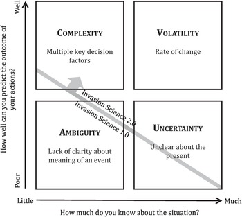
Figure 1.24 Invasion science in a VUCA world. By defining and unifying terminology, metrics and frameworks, invasion science has largely rooted out ambiguity in the field. However, work is still underway to reduce uncertainty associated with the current knowledge of invasion status and the ecology of invasive species. Future work must embrace complexity in invasion science, both in terms of ecosystems and multiple stakeholders, while volatility in invasion science has yet to truly emerge, as the rate of invasions and their impacts are currently increasing unabated, although critics have started sounding alarms.

In the following chapters we move tentatively into the Complexity component by approaching it as an ecological network facing biological invasions. This resonates with the paradigm shift in human knowledge systems from the classic tree structures to the emerging network metaphor (Lima 2015). How does a non-native species invade an ecological network? Which aspects and components of the network should concern us? In network science, a complex network normally possesses five features: interdependence (watch out for knock-on effects), interconnectivity (six-degree; all connected eventually), decentralisation (lack of governance), multiplicity (exponential/explosive) and non-linearity (1+1 is not 2; feedbacks). Interdependence describes the interactions between connected nodes in a network; interconnectivity portrays the emerged network structures and architectures; decentralisation depicts the function and regime/stability of a network; multiplicity talks about the dynamics of nodes in a network; non-linearity characterises the response of a network to invasions (i.e., invasibility). For an ecological network affected by biological invasions, we not only dissect the system into these five aspects but also address the issue of scale. We devote full chapters to, in sequence, network interactions, network patterns, network stability, network dynamics, network scaling and network invasibility. Again, this is not a recipe book but an atlas of clues and ideas for the roads ahead. Please fasten your seatbelts. Bon voyage.